The goal of social science research
Use data to discover patterns ("social facts" in Durkheim's terms),
and the social mechanisms that bring them about.

Remember RCTs!

- If we randomly divide subjects into treatment and control groups: They come from the same underlying population.
Similar on average, in every way,
including their !
!
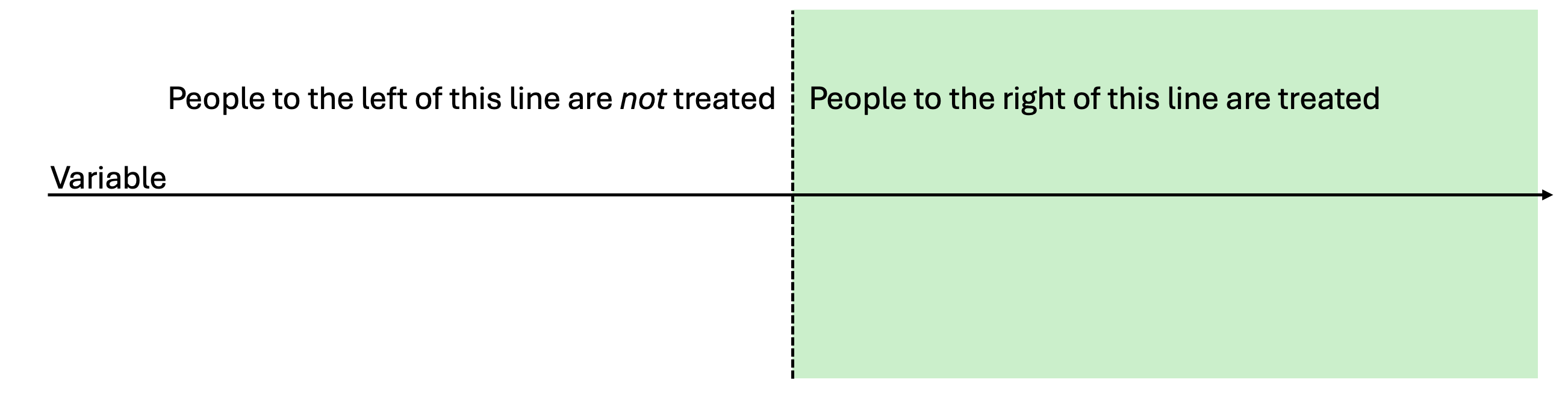
RDD Intuitions
What if we compared people who fall right on either side of the threshold?
- Assignment isn't random
- But right at the threshold, maybe it's close to random?
RDD Intuitions
But which group you fall into becomes less random the further you get from the threshold
- Someone who loses an election badly is probably very different from a person who loses an election by a few votes
- Someone who is 23 is probably very different from a person who is 64
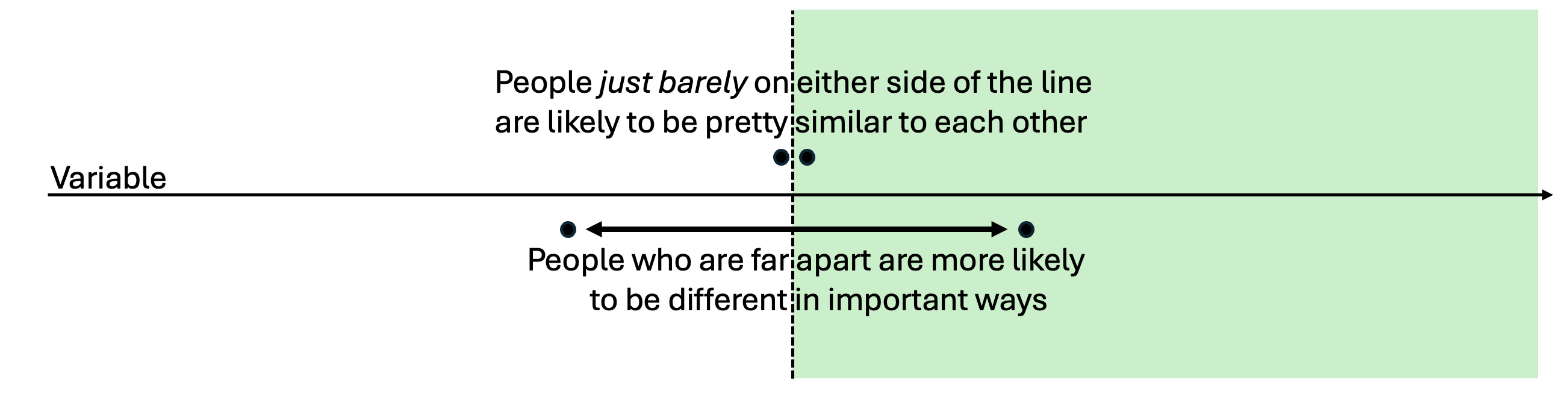
RDD Intuitions
So we would really like to compare people just barely on either side of the threshold
How can we make this work? An Example

How can we make this work? An Example
What is the causal effect of
making alcohol consumption legal
on mortality?
Let's try our idea
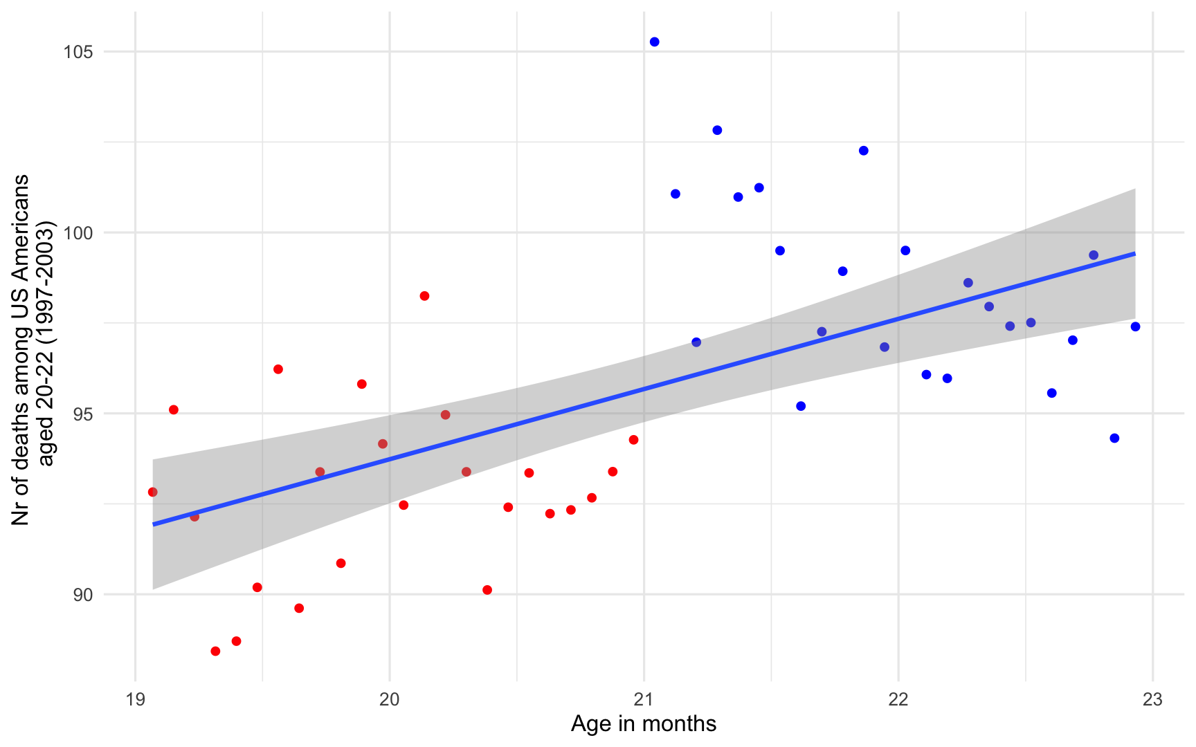
Let's compare those who are legally too young to drink (>21) to those who are old enough to drink?
pacman::p_load( tidyverse, # Data manipulation, ggplot2, # beautiful figures, estimatr, # OLS with robust SE texreg, # regression tables with nice layout, rdrobust, # Non-parametric regression, RDDtools # easy RDD fitting)# Get the Minimum legal drinking age data!data("mlda", package = "masteringmetrics")mlda <- mlda %>% drop_na()mlda # print the tibble.# # A tibble: 48 × 19# agecell all allfitted internal internalfitted external externalfitted alcohol alcoholfitted homicide# <dbl> <dbl> <dbl> <dbl> <dbl> <dbl> <dbl> <dbl> <dbl> <dbl># 1 19.1 92.8 91.7 16.6 16.7 76.2 75.0 0.639 0.794 16.3# 2 19.2 95.1 91.9 18.3 16.9 76.8 75.0 0.677 0.838 16.9# 3 19.2 92.1 92.0 18.9 17.1 73.2 75.0 0.866 0.878 15.2# 4 19.3 88.4 92.2 16.1 17.3 72.3 74.9 0.867 0.915 16.7# 5 19.4 88.7 92.3 17.4 17.4 71.3 74.9 1.02 0.949 14.9# 6 19.5 90.2 92.5 17.9 17.6 72.3 74.9 1.17 0.981 15.6# 7 19.6 96.2 92.6 16.4 17.8 79.8 74.8 0.870 1.01 16.3# 8 19.6 89.6 92.7 16.0 17.9 73.6 74.8 1.10 1.03 15.8# 9 19.7 93.4 92.8 17.4 18.1 75.9 74.7 1.17 1.06 16.8# 10 19.8 90.9 92.9 18.3 18.2 72.6 74.6 0.948 1.08 16.6# # ℹ 38 more rows# # ℹ 9 more variables: homicidefitted <dbl>, suicide <dbl>, suicidefitted <dbl>, mva <dbl>, mvafitted <dbl>,# # drugs <dbl>, drugsfitted <dbl>, externalother <dbl>, externalotherfitted <dbl>- Everything on this slide and the next is done with tidyverse and ggplot2
- Later we will use the RDDtools package to do the more complex tasks
- When we do that, it will be much easier to use the plot() command instead of ggplot2
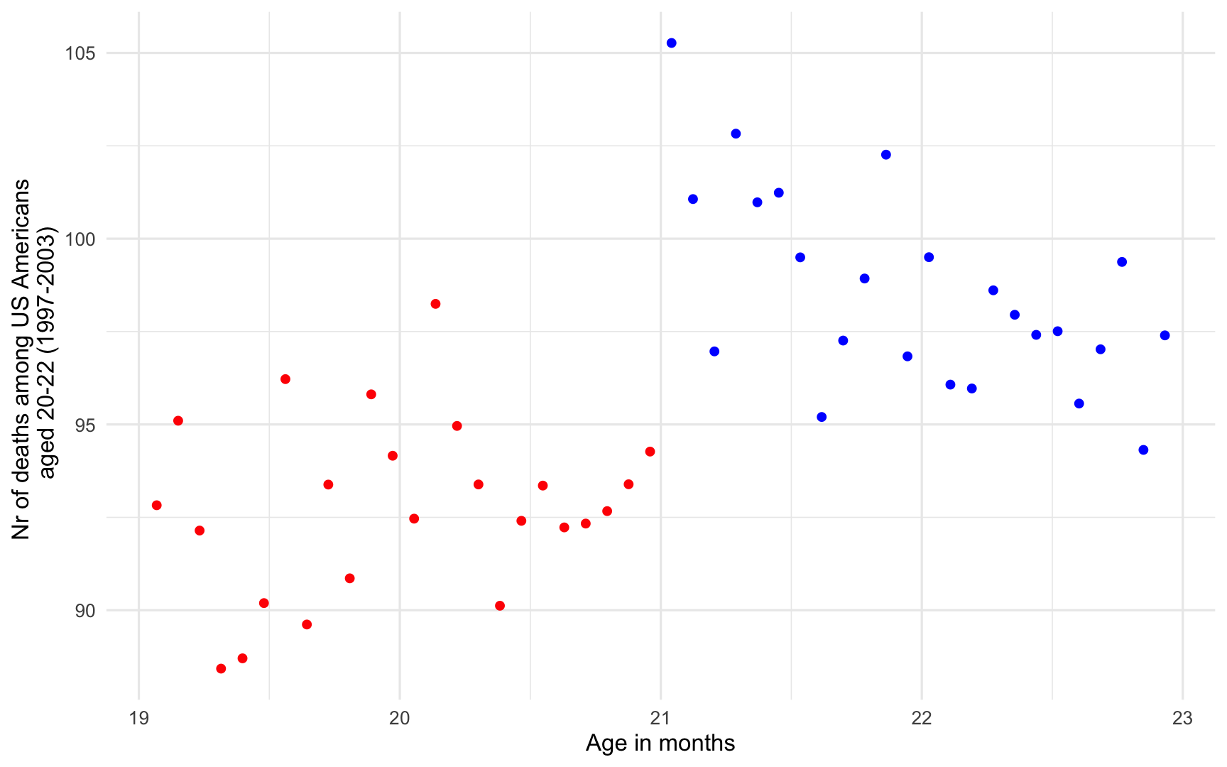
mlda <- mlda %>% mutate( # Define those who are allowed to drink over21 = case_when( agecell >= 21 ~ "Yes", TRUE ~ "No") )ggplot(data = mlda, aes(y = all, x = agecell, color = over21)) + geom_point() + theme_minimal() + scale_color_manual(values = c("red", "blue")) + labs(y = "Nr of deaths among US Americans \n aged 20-22 (1997-2003)", x = "Age in months") + guides(color = "none")Let's try our idea
So now let's zoom in on the data right around the threshold
mlda <- mlda %>% mutate( # Define those who are allowed to drink close = case_when( agecell >= 20.7 & agecell < 21 ~ "low", agecell >= 21 & agecell < 21.3 ~ "high", TRUE ~ "No"))ggplot(data = mlda, aes(y = all, x = agecell, color = close)) + geom_point() + theme_minimal() + scale_color_manual(values = c("blue", "red", "black")) + labs(y = "Nr of deaths among US Americans \n aged 20-22 (1997-2003)", x = "Age in months") + guides(color = "none")
Implementation
Parametric RDD with RDDtools
Using the R package RDDtools, we can implement all of these models rather easily. The main challenge is just to install it. See Exercise 1 on that point.
First, creating a plot of the discontinuity with RDDtools
# Tell the package that it is an RDD dataset# y = the Y variable of interest, in this case mlda$all# x = the X variable of interest, in this case mlda$agecell# cutpoint = the point of discontinuity in the data, in this case 21drinking_rdd_data <- RDDdata( y=mlda$all, x=mlda$agecell, cutpoint=21 )# Note that this renames the variables to y and x. Do not be alarmed.# And do not change the variable names back, or you will get error messages

# It's helpful to change the axis labels since it changes the variable names# and 'x' and 'y' aren't very informativeplot( drinking_rdd_data, xlab='Age in months\n', # A little extra white space ylab="Nr of deaths among US Americans aged 20-22 (1997-2003)" )Implementation
Parametric RDD with RDDtools
Using the R package RDDtools, we can implement all of these models rather easily. The main challenge is just to install it. See Exercise 1 on that point.
Next, creating a simple linear model without any polynomial terms
# Order refers to the polynomial. Polynomials of order 1 are just normal variables# without any exponents.# Slope can be set to "same" if we want both sides of the threshold to have the same# slope. It can also be set to "separate" if we want to add an interaction term so as# to allow the slopes on each side to differ from one another, as described in the textbook.rdd_linear <- RDDreg_lm( RDDobject = drinking_rdd_data, order = 1, slope='same' )summary(rdd_linear)# # Call:# lm(formula = y ~ ., data = dat_step1, weights = weights)# # Residuals:# Min 1Q Median 3Q Max # -5.056 -1.848 0.115 1.491 5.804 # # Coefficients:# Estimate Std. Error t value Pr(>|t|) # (Intercept) 91.841 0.805 114.08 < 2e-16 ***# D 7.663 1.440 5.32 3.1e-06 ***# x -0.975 0.632 -1.54 0.13 # ---# Signif. codes: 0 '***' 0.001 '**' 0.01 '*' 0.05 '.' 0.1 ' ' 1# # Residual standard error: 2.49 on 45 degrees of freedom# Multiple R-squared: 0.595, Adjusted R-squared: 0.577 # F-statistic: 33 on 2 and 45 DF, p-value: 1.51e-09

# It's helpful to change the axis labels since it changes the variable names# and 'x' and 'y' aren't very informativeplot( rdd_linear, xlab='Age in months\n', # A little extra white space ylab="Nr of deaths among US Americans aged 20-22 (1997-2003)" )Implementation
Parametric RDD with RDDtools
Using the R package RDDtools, we can implement all of these models rather easily. The main challenge is just to install it. See Exercise 1 on that point.
Finally, adding in some polynomial terms (power of 2)
# Order refers to the polynomial. Polynomials of order 1 are just normal variables# without any exponents.# Slope can be set to "same" if we want both sides of the threshold to have the same# slope. It can also be set to "separate" if we want to add an interaction term so as# to allow the slopes on each side to differ from one another, as described in the textbook.rdd_quadratic <- RDDreg_lm( RDDobject = drinking_rdd_data, order = 2, slope='same' )summary(rdd_quadratic)# # Call:# lm(formula = y ~ ., data = dat_step1, weights = weights)# # Residuals:# Min 1Q Median 3Q Max # -4.45 -1.75 0.19 1.16 5.11 # # Coefficients:# Estimate Std. Error t value Pr(>|t|) # (Intercept) 92.903 0.837 110.99 < 2e-16 ***# D 7.663 1.339 5.72 8.7e-07 ***# x -0.975 0.588 -1.66 0.1046 # `x^2` -0.819 0.289 -2.84 0.0069 ** # ---# Signif. codes: 0 '***' 0.001 '**' 0.01 '*' 0.05 '.' 0.1 ' ' 1# # Residual standard error: 2.32 on 44 degrees of freedom# Multiple R-squared: 0.657, Adjusted R-squared: 0.634 # F-statistic: 28.1 on 3 and 44 DF, p-value: 2.61e-10

# It's helpful to change the axis labels since it changes the variable names# and 'x' and 'y' aren't very informativeplot( rdd_quadratic, xlab='Age in months\n', # A little extra white space ylab="Nr of deaths among US Americans aged 20-22 (1997-2003)" )Time to try Exercise #1

Reminder!
We would really like to compare people just barely on either side of the threshold
But so far we are using all the data points, and using polynomials to home in on real effect with our estimates. This lets us keep all the data, which gives us more statistical power. But there is an alternative.
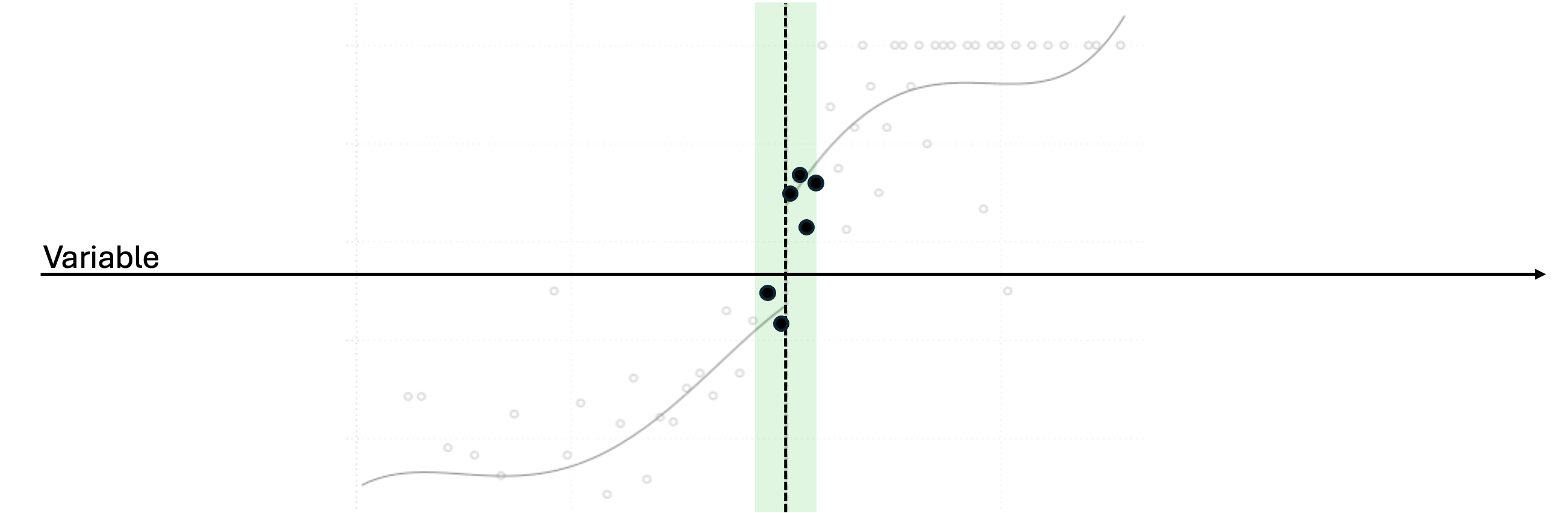
Nonparametric RDD
How do we balance the "bandwidth"
If we draw the green box too small (too close to the threshold), we will lose statistical power and won't be able to draw meaningful conclusions. If we draw the green box too big, we get more observations, but we lose the strength of the comparison. We call the width of the box the "bandwidth"
Nonparametric RDD
That is, we want to estimate this:
But we only want to estimate it in a sample where:
Empirical example #1
Women and corruption
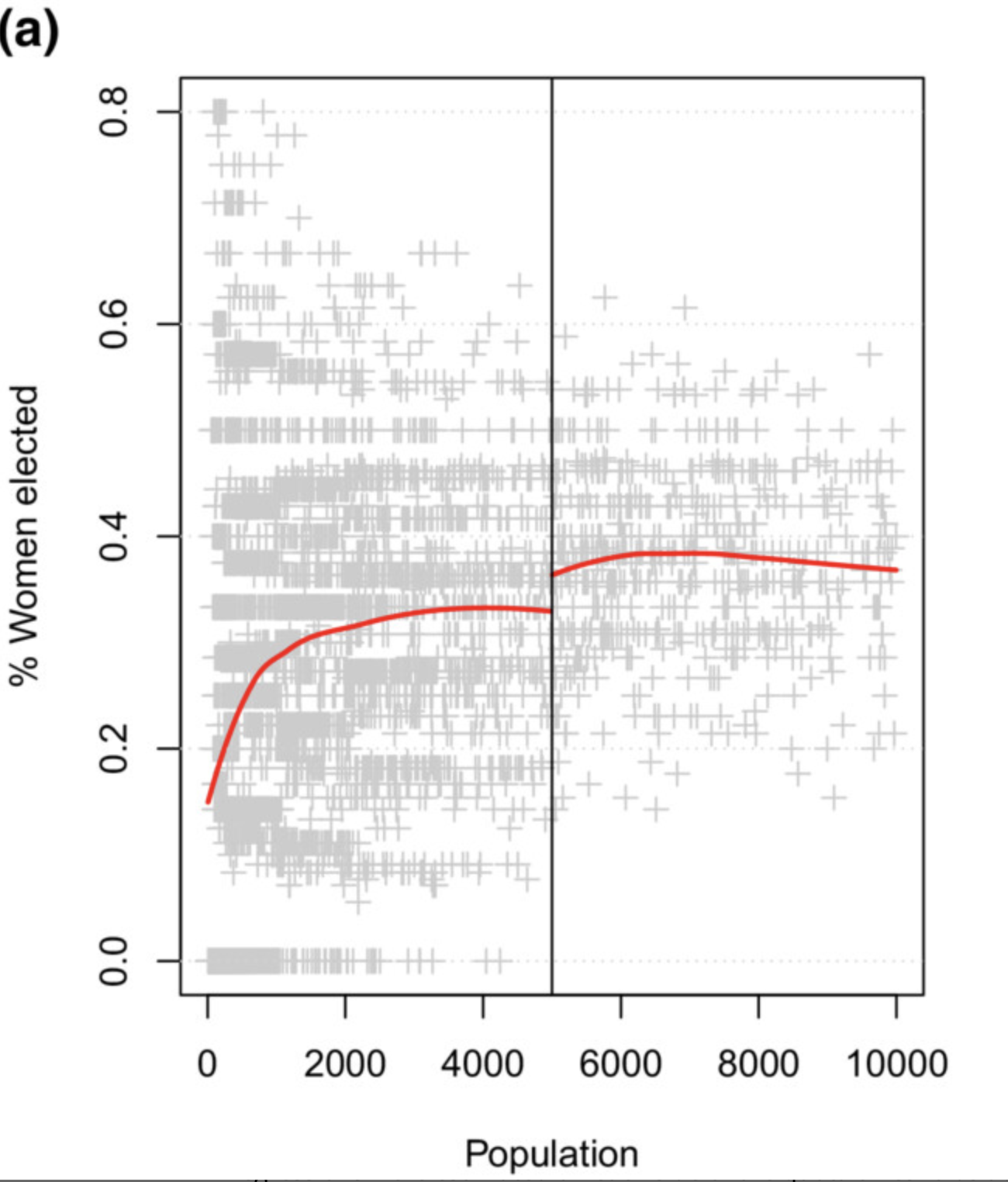
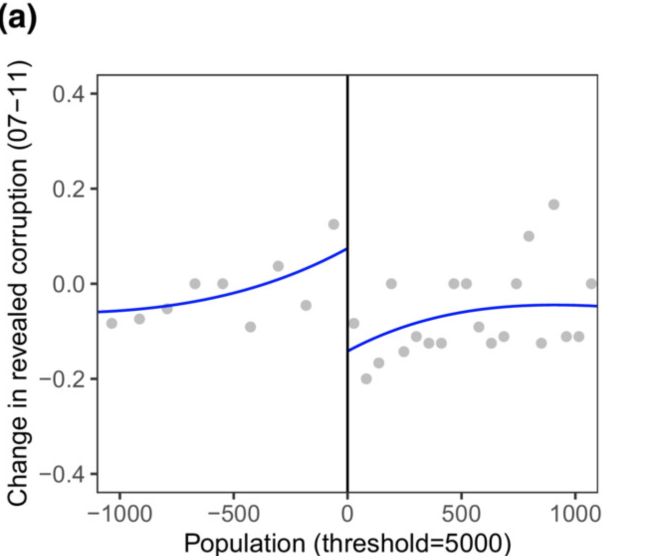
In 2007 Spain made a new rule saying that for towns with a population larger than 5000 people, parties had to provide at least 40% of their seats to women. They use this as an RDD to look into the well-known correlation between women in government and corruption.
Empirical example #1
Women and corruption
There's an effect! But why?
Empirical example #1
Women and corruption
There's an effect! But why?
- Women are socialized differently
- Women are more risk averse
- Women are under more scrutiny when elected
- Women tend to work on policies in low-corruption areas
Empirical example #2
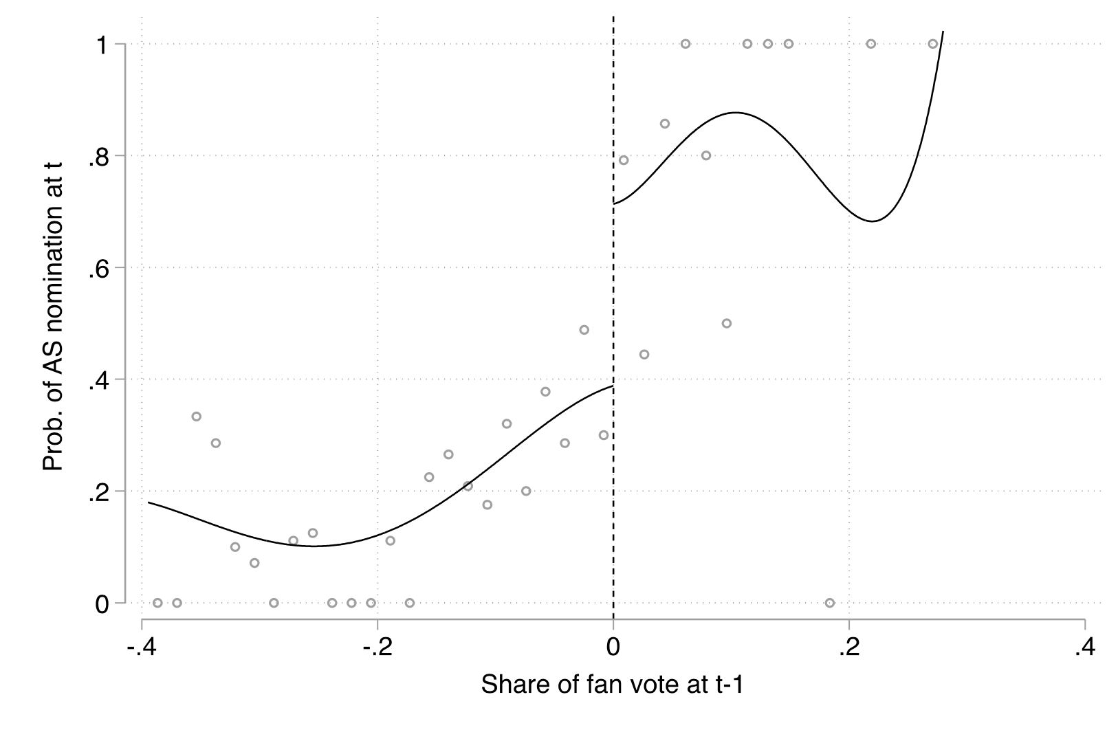
Cumulative advantage in basketball
- Fans vote to decide who plays in the NBA "All-Star Game"
- People in the Top X players at each position get to play
- People with just a few votes less do not get to play
Does winning the fan vote in time t increase a person's chances of winning the fan vote again in time t+1 and beyond?

Empirical example #2
Cumulative advantage in basketball
There's an effect! But why?
Sociologist Robert Merton argued that this happens because we don't have enough available space to reward every deserving person (in his case, it was scientists...think the Nobel prize). We have to make decisions between people who are more or less equal, and rewarding one person at the threshold but not the other creates an actual inequality where there didn't use to be any.
]
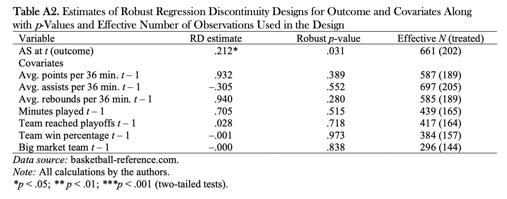
Empirical example #2
Cumulative advantage in basketball
Maybe the players who won the first time are just better? Nope. Every measure of performance is insignificant, while the RDD estimate remains significant.
Empirical example #2
Far-right elections and welfare chauvisnism
I can't show you the evidence, because it isn't published yet! But I saw your professor present this work in Leipzig.
Newly arrived residents of Italian regions that just barely elect far-right governments are more likely to experience delays and difficulties getting their healthcare access set up, compared to those who live in regions that just barely did not elect far-right governments.

Time to try Exercise #2