Multiple OLS in Practice

Confounders, mediators, and controls you can’t measure

Merlin Schaeffer · Department of Sociology

2026-07-23

By the end of today you can …

1. tell a confounder from a mediator on a causal diagram — and know that you control the first but usually not the second;

2. read a multiple regression coefficient as “holding the other variables constant” — and see how it does that (Frisch–Waugh);

3. use a smart summary control to stand in for confounders you cannot measure.

One part per goal. Two running questions: the gender pay gap in Denmark, and — back to Lecture 2 — does state ownership of the economy reduce poverty?

By now they can run a multiple regression; today is about deciding what belongs in it. Set the stakes early: adding a variable is not a neutral act — the same command can repair a comparison or quietly destroy it. Two running examples today, and one of them picks Lecture 2 back up.

Confounders vs. mediators

Part 1 of 2

Adding a variable to a regression can sharpen a comparison — or quietly ruin it. The difference is the arrow’s direction.

Two jobs for a control variable

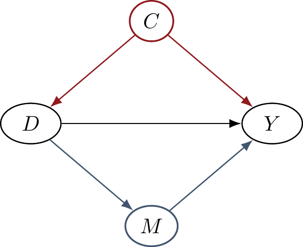
Confounder \(C\) (red) — sits on a backdoor path: an arrow runs into the treatment \(D\) and into the outcome \(Y\).

\(\rightarrow\) Control it. Multiple OLS blocks the backdoor and makes the comparison fairer.

Mediator \(M\) (blue) — sits on the causal path \(D \rightarrow M \rightarrow Y\): an arrow runs out of the treatment.

\(\rightarrow\) Usually leave it in. Controlling a mediator removes part of the very effect you want.

This one DAG is the whole first half. Make them read the arrowheads, not the positions: the confounder has an arrow running into the treatment, the mediator has one running out of it. Same shape on the page, opposite advice. If they can tell these apart on an exam DAG, today has worked.

Why the direction matters

To get closer to the overall causal effect \(D \rightarrow Y\), control observed confounders — but never control a mediator: you would throw away the part of the effect that runs through it.

The exception is deliberate: sometimes we want the partial effect of \(D\) that does not run through \(M\) — then controlling \(M\) is exactly the point. Know which question you are asking.

Resist giving them a rule to memorise. “Never control a mediator” is the default, but the blue box is the honest version: sometimes the partial effect is the question. The discipline is not knowing the rule, it is knowing which question you asked before you typed the formula.

A clear case of mediation

• The question
• The data
• The models
• The verdict

Danish women earn less per month than Danish men. How much of that gap is because women more often work fewer contracted hours?

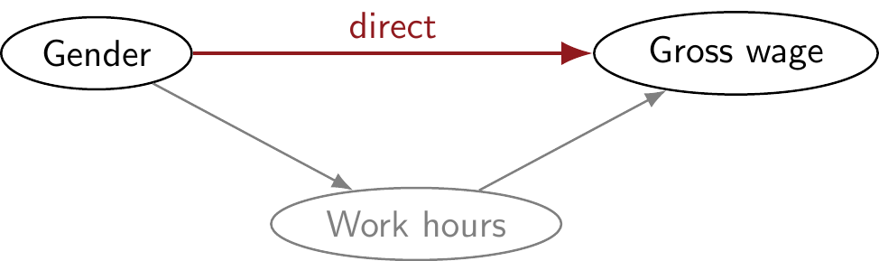
Work hours is a mediator: gender shapes hours, and hours shape pay.

pacman::p_load(tidyverse, haven, estimatr, modelsummary)

# ESS round 9, Denmark. Monthly gross wage, gender, contracted work hours.
ESS <- read_spss("../assets/ESS9e03_1.sav") %>%
  filter(cntry == "DK") %>%
  select(pspwght, gndr, wkhct, grspnum, infqbst) %>%
  mutate(
    across(c(pspwght, wkhct, grspnum), zap_labels),
    gndr   = as_factor(gndr),
    grwage = case_when(          # Put everyone on a monthly basis
      infqbst == 1 ~ 4 * grspnum,   # weekly  -> monthly
      infqbst == 3 ~ grspnum / 12,  # yearly  -> monthly
      TRUE         ~ grspnum        # already monthly
    )
  ) %>%
  filter(wkhct > 0) %>%
  drop_na()

mod1 <- lm_robust(grwage ~ gndr,         data = ESS, weights = pspwght)
mod2 <- lm_robust(grwage ~ gndr + wkhct, data = ESS, weights = pspwght)

modelsummary(
  list("Gross wage" = mod1, "Gross wage" = mod2),
  coef_rename = c("gndrFemale" = "Female", "wkhct" = "Weekly hours"),
  stars = TRUE, gof_map = c("nobs", "r.squared"),
  output = "kableExtra"
)

	Gross wage	Gross wage
(Intercept)	41997.795***	6778.675
	(4727.672)	(5160.501)
Female	−9492.532+	−6096.550
	(5174.552)	(5106.762)
Weekly hours		977.304***
		(99.479)
Num.Obs.	778	778
R2	0.003	0.011
+ p < 0.1, * p < 0.05, ** p < 0.01, *** p < 0.001

The raw gap of 9,493 kr./month shrinks to 6,097 kr. once we hold work hours constant: about 36% of the gender pay gap runs through fewer contracted hours. The rest does not — and controlling hours would hide it.

An unambiguous mediator, so use it to build confidence: gender cannot be caused by working hours, the arrow only runs one way. Ask them to predict what happens to the gap before you show the second column. Then the interpretation that matters — the shrinkage is not a nuisance, it is the finding: about a third of the gap is the hours. And note what the remaining gap means: equal contracted hours, still unequal pay.

An unclear case — back to Lecture 2

In Lecture 2 we asked: do state-owned (socialist) economies reduce poverty? Descriptively — no. But they also offer fewer civil liberties, and civil liberties themselves predict less poverty.

Discuss: are civil liberties a confounder or a mediator of the state ownership → poverty relationship? Should we control for them?

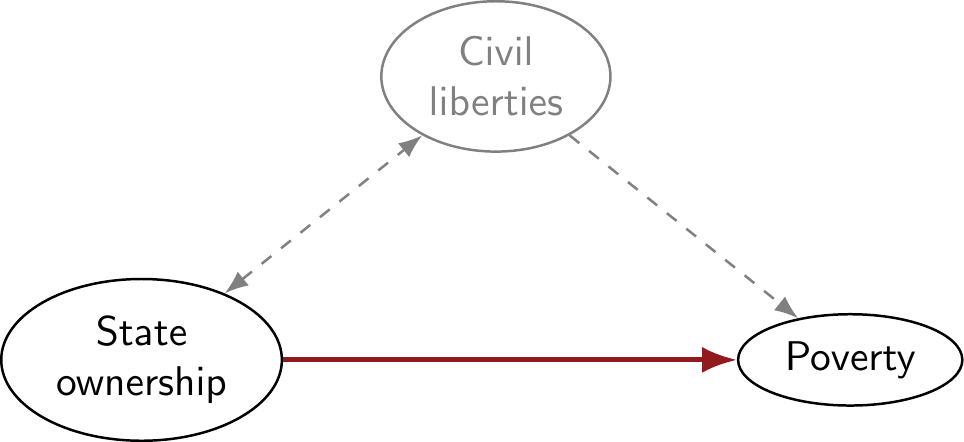
The double-headed dashed arrow is the honest part: with cross-country data we cannot be sure whether fewer civil liberties cause state ownership or the reverse.

Now the hard case, and there is no clean answer — say that up front. Let them argue both readings: civil liberties as a confounder (regimes that restrict liberties also nationalise) or as a mediator (state ownership erodes liberties). Point at the double-headed arrow: with cross-country data we genuinely cannot settle the direction. The honest move is to change the question, which is the next slide.

The revised research question

Would state-owned economies reduce poverty more — if they did not also curb their citizens’ civil liberties?

That is the partial effect of state ownership that does not run through civil liberties. Multiple OLS can estimate it.

This is the move worth teaching: when you cannot resolve the DAG, sharpen the question until your model answers something you can actually defend. We are no longer claiming the total effect — we are asking about the part that does not run through civil liberties. Say the revised question slowly; they will need it to read the next table honestly.

Preparation

• Packages
• Get & join the data

pacman::p_load(
  tidyverse,    # Data manipulation and visualization
  wbstats,      # World Bank data via API
  vdemdata,     # Varieties of Democracy (V-Dem) data
  estimatr,     # OLS with robust standard errors
  modelsummary  # Regression tables
)

# V-Dem: civil liberties (equality before the law and individual liberty) and state ownership
Dat_vdem <- vdem %>%
  as_tibble() %>%
  select(country_text_id, year,
         civ_liberties = v2xcl_rol,
         state_own_raw   = v2clstown) %>%
  mutate(state_ownership = -state_own_raw) # Reverse: higher = MORE state ownership

# World Bank: extreme poverty (< $3.00 a day). Live, with cached fallback.
Dat_poverty <- tryCatch(
  wb_data("SI.POV.DDAY", start_date = 1972, end_date = 2025),
  error = function(e) readRDS("data/wb_poverty_raw.rds")
) %>%
  rename(poverty = SI.POV.DDAY, year = date, country_text_id = iso3c) %>%
  select(country_text_id, year, country, poverty) %>%
  drop_na(poverty) %>%
  group_by(country) %>% filter(year == max(year)) %>% ungroup()

(Dat <- inner_join(Dat_poverty, Dat_vdem,
                   by = c("country_text_id", "year")) %>%
   drop_na(poverty, state_ownership, civ_liberties))
# # A tibble: 161 × 7
#    country_text_id  year country    poverty civ_liberties state_own_raw state_ownership
#    <chr>           <dbl> <chr>        <dbl>         <dbl>         <dbl>           <dbl>
#  1 ALB              2020 Albania        0.3         0.914         1.57           -1.57 
#  2 DZA              2011 Algeria        0           0.575        -1.91            1.91 
#  3 AGO              2018 Angola        39.3         0.559        -0.746           0.746
#  4 ARG              2024 Argentina      1           0.844         1.39           -1.39 
#  5 ARM              2024 Armenia        0.8         0.839         1.64           -1.64 
#  6 AUS              2020 Australia      0.9         0.949         1.44           -1.44 
#  7 AUT              2023 Austria        0.5         0.937         0.479          -0.479
#  8 AZE              2005 Azerbaijan     0           0.38         -0.617           0.617
#  9 BGD              2022 Bangladesh     5.9         0.338         0.371          -0.371
# 10 BRB              2016 Barbados       1.7         0.919         0.753          -0.753
# # ℹ 151 more rows

Multiple OLS: one control changes everything

# Bivariate: state ownership only
ols <- lm_robust(poverty ~ state_ownership, data = Dat)

# Multiple: add civil liberties
ols_mult <- lm_robust(
  poverty ~ state_ownership + civ_liberties,
  data = Dat
)

modelsummary(
  list("Poverty" = ols, "Poverty" = ols_mult),
  coef_rename = c("state_ownership" = "State ownership",
                  "civ_liberties" = "Civil liberties"),
  stars = TRUE, gof_map = c("nobs", "r.squared"),
  output = "kableExtra"
)

	Poverty	Poverty
(Intercept)	15.914***	37.041***
	(2.166)	(6.020)
State ownership	2.742	−3.781+
	(1.705)	(2.058)
Civil liberties		−37.012***
		(8.501)
Num.Obs.	161	161
R2	0.017	0.124
+ p < 0.1, * p < 0.05, ** p < 0.01, *** p < 0.001

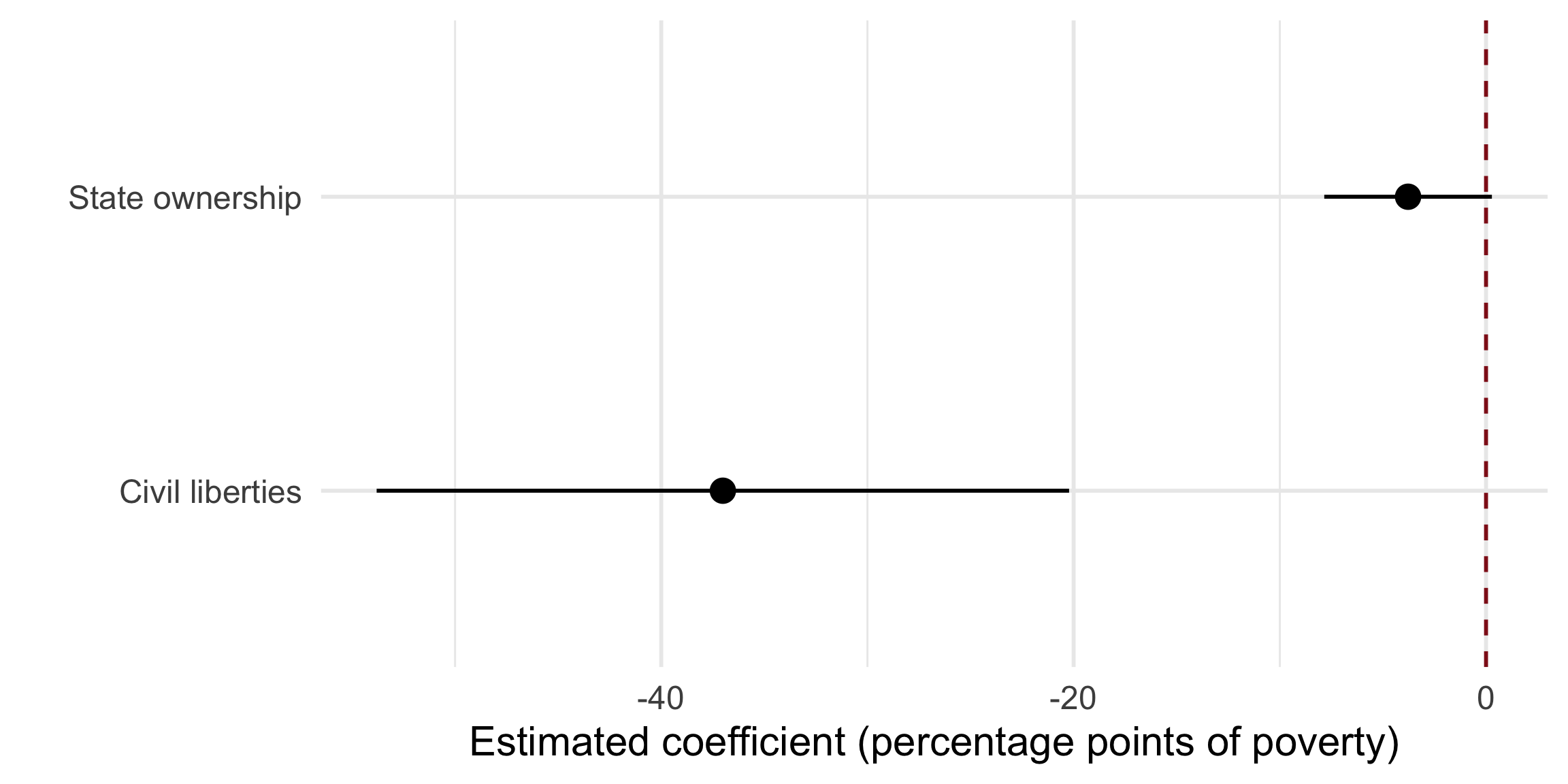
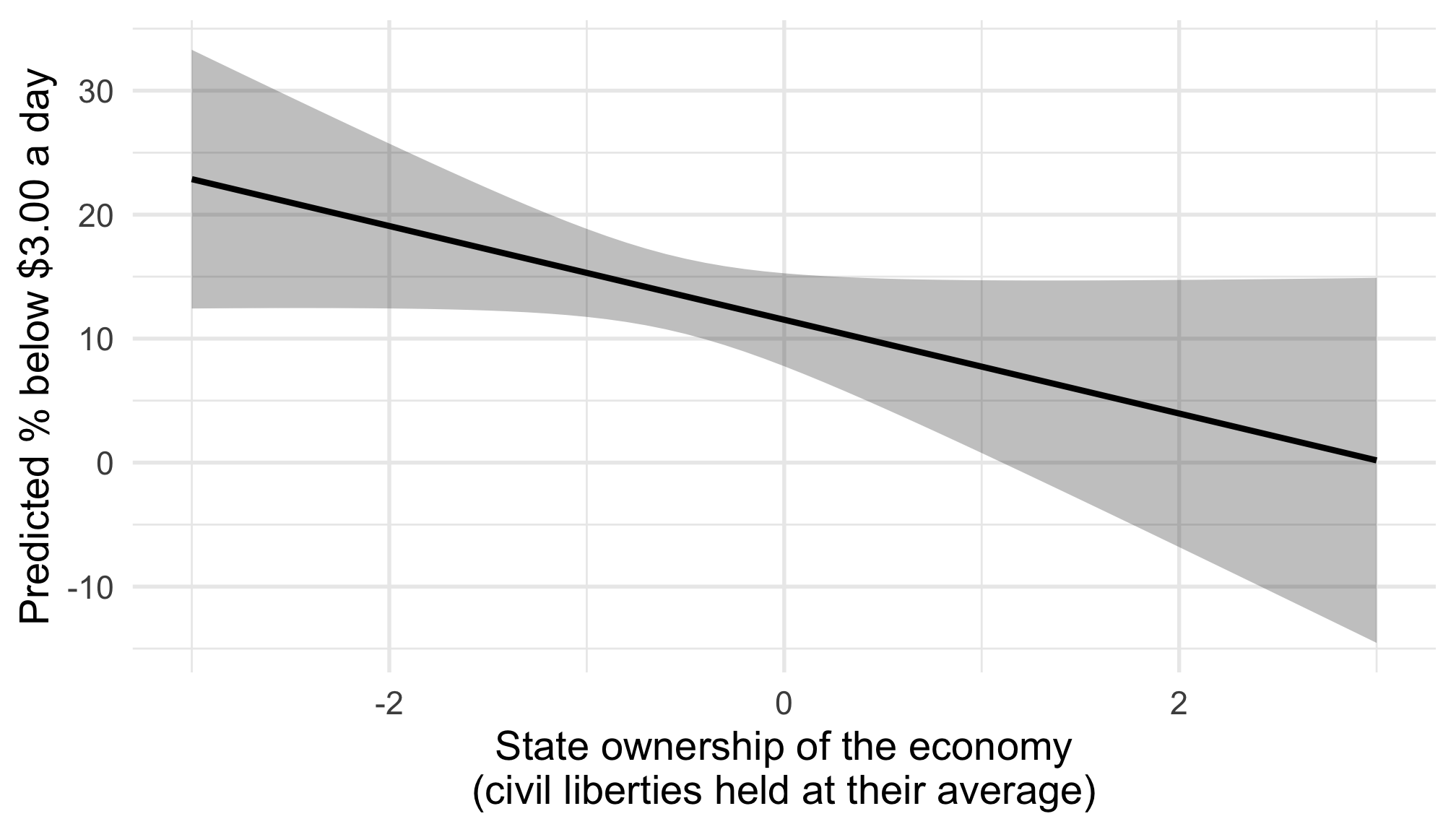
On its own, state ownership looks harmless. Holding civil liberties constant, its sign flips — among countries with the same civil liberties, more state ownership goes with less poverty. Civil liberties were masking it.

Show column one, ask them to predict column two, then reveal. A sign flip is dramatic and they will remember it — but immediately supply the careful reading: not “state ownership reduces poverty”, but “among countries with the same civil liberties, more state ownership goes with less poverty”. Same data, one extra column, opposite story. Nothing here is causal, and the comparison is only fairer, not fair.

What does “holding constant” actually do?

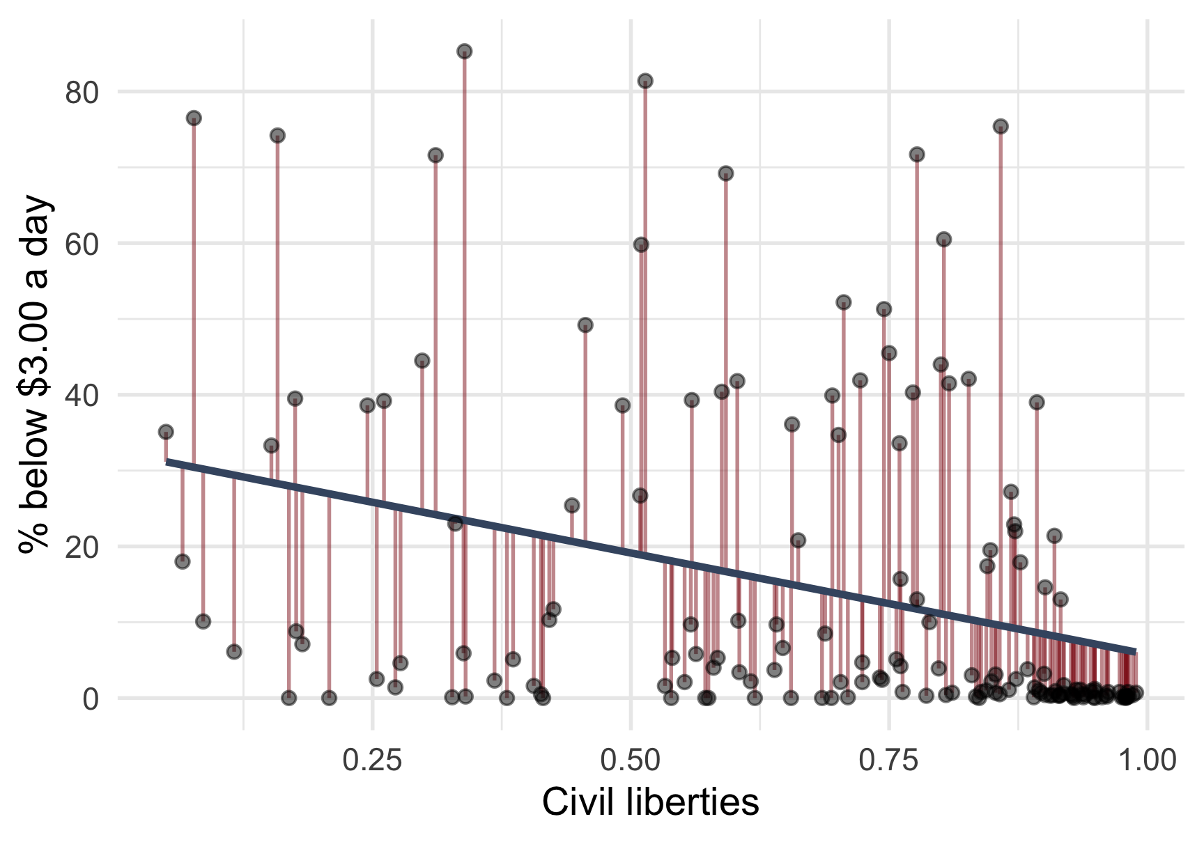
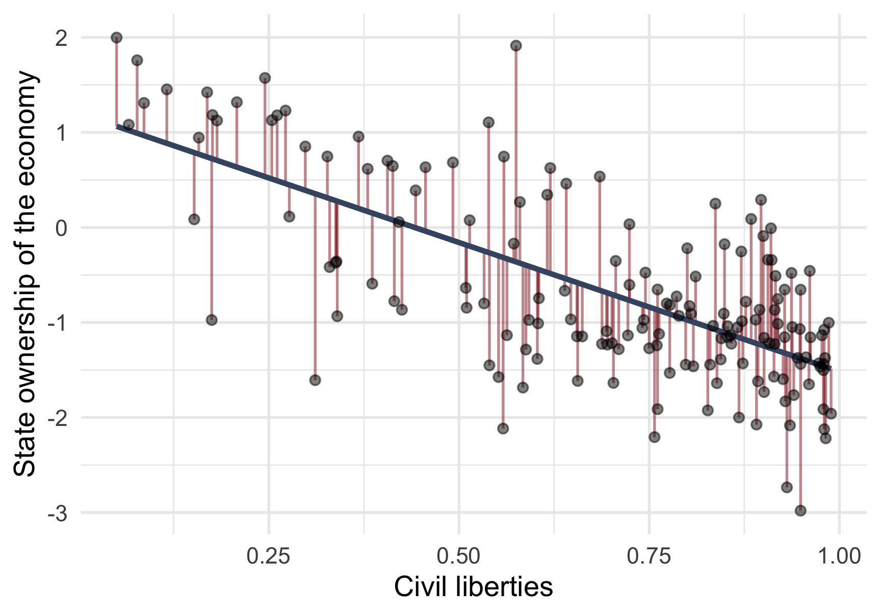
Frisch and Waugh (1933) showed that “controlling for” a variable is exactly a three-step residualisation — regression by subtraction.

Frisch–Waugh, step 1

Regress the outcome on the control, keep the residuals — the part of poverty that civil liberties do not explain.

Dat <- Dat %>%
  add_residuals(
    model = lm(poverty ~ civ_liberties, data = .),
    var   = "e_poverty"
  )

Frame the three steps before starting step 1: we are going to earn the phrase “holding constant” instead of just saying it. Step 1 strips civil liberties out of poverty — the red lines are what is left over, the part civil liberties cannot explain. Keep the pace brisk; the payoff is step 3.

Frisch–Waugh, step 2

Regress the treatment on the control, keep the residuals — the part of state ownership that civil liberties do not explain.

Dat <- Dat %>%
  add_residuals(
    model = lm(state_ownership ~ civ_liberties, data = .),
    var   = "e_stateown"
  )

Exactly the same operation, now on the treatment: strip civil liberties out of state ownership. What remains is variation in state ownership that has nothing to do with civil liberties. Point out that both variables have now been cleaned with the same rag — that symmetry is why the next step works.

Frisch–Waugh, step 3

Regress the two sets of residuals on each other. Its slope is identical to the multiple-regression coefficient.

ols_resid <- lm_robust(e_poverty ~ e_stateown, data = Dat)

modelsummary(
  list("Multiple OLS" = ols_mult,
       "Residualised" = ols_resid),
  coef_rename = c("state_ownership" = "State ownership",
                  "civ_liberties" = "Civil liberties",
                  "e_stateown" = "State ownership (resid.)"),
  coef_omit = "(Intercept)",
  stars = TRUE, gof_map = c("nobs"),
  output = "kableExtra"
)

	Multiple OLS	Residualised
State ownership	−3.781+
	(2.058)
Civil liberties	−37.012***
	(8.501)
State ownership (resid.)		−3.781+
		(2.049)
Num.Obs.	161	161
+ p < 0.1, * p < 0.05, ** p < 0.01, *** p < 0.001

Same number, two routes: the residualised slope on e_stateown equals the multiple model’s state_ownership coefficient. That is all controlling for civil liberties does.

The payoff — let them see the two coefficients match to the decimal before you say anything. Then the point: multiple regression is not doing anything mysterious, it is subtracting away the control from both variables and fitting a simple line to what is left. “Holding constant” now has a mechanism, not just a phrase.

Show the result

• Coefficient plot
• Predictions

To predict, set the control to an informative constant (here: average civil liberties), then vary the treatment.

Two ways to show the same model — they will need both for the exam and for exercise 2. On the prediction plot, stress the choice hiding in the code: you must pin the control somewhere, and we pinned civil liberties at their average. Different choice, different line — so always say where you pinned it.

Break

Your turn: exercise 1

You practice multiple OLS on the carbon divide from Lecture 4: do regions differ in emissions beyond their wealth?

Open exercise 1 in a new tab ↗

Smart summary controls

Part 2 of 2

“To control for a wide range of factors seems daunting: the possibilities are virtually infinite, and many characteristics are hard to quantify.”

— Angrist and Pischke (2014, p. 51)

Read the Angrist quote out loud — it names the anxiety they should be feeling by now. If good inference means controlling for everything, and the list is infinite and half of it unmeasurable, the project looks hopeless. Part 2 is the escape: sometimes one cleverly chosen variable stands in for the whole list.

Football and domestic violence

Discuss: what confounds the effect of a team losing on domestic violence? (Team quality, the kind of fan, the kind of city …) How could a single variable stand in for all of them?

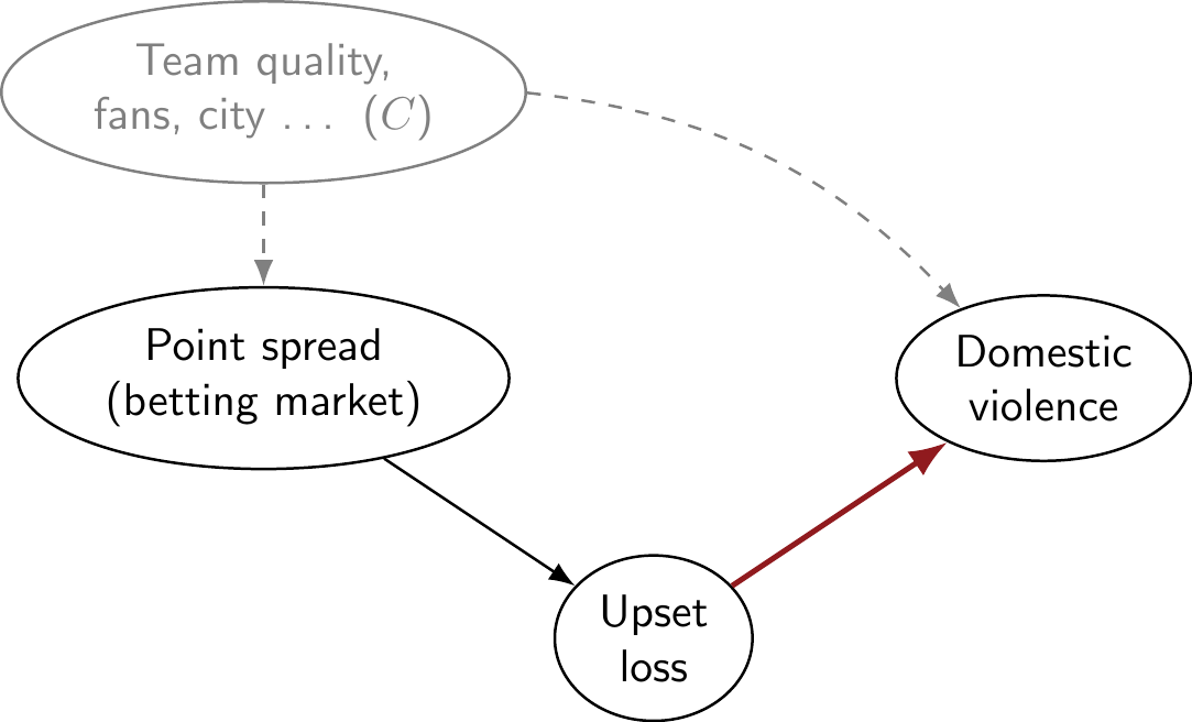
The point spread already prices in everything the market knows about both teams — one number that summarises a world of confounders (Card and Dahl, 2011).

Let them brainstorm confounders first — they will produce team quality, kind of fan, kind of city, and quickly run out of measurable ones. Then the trick: a betting market has already done that work, because thousands of people with money at stake priced every one of those factors into a single number. One column standing in for a list nobody could finish.

Football and domestic violence

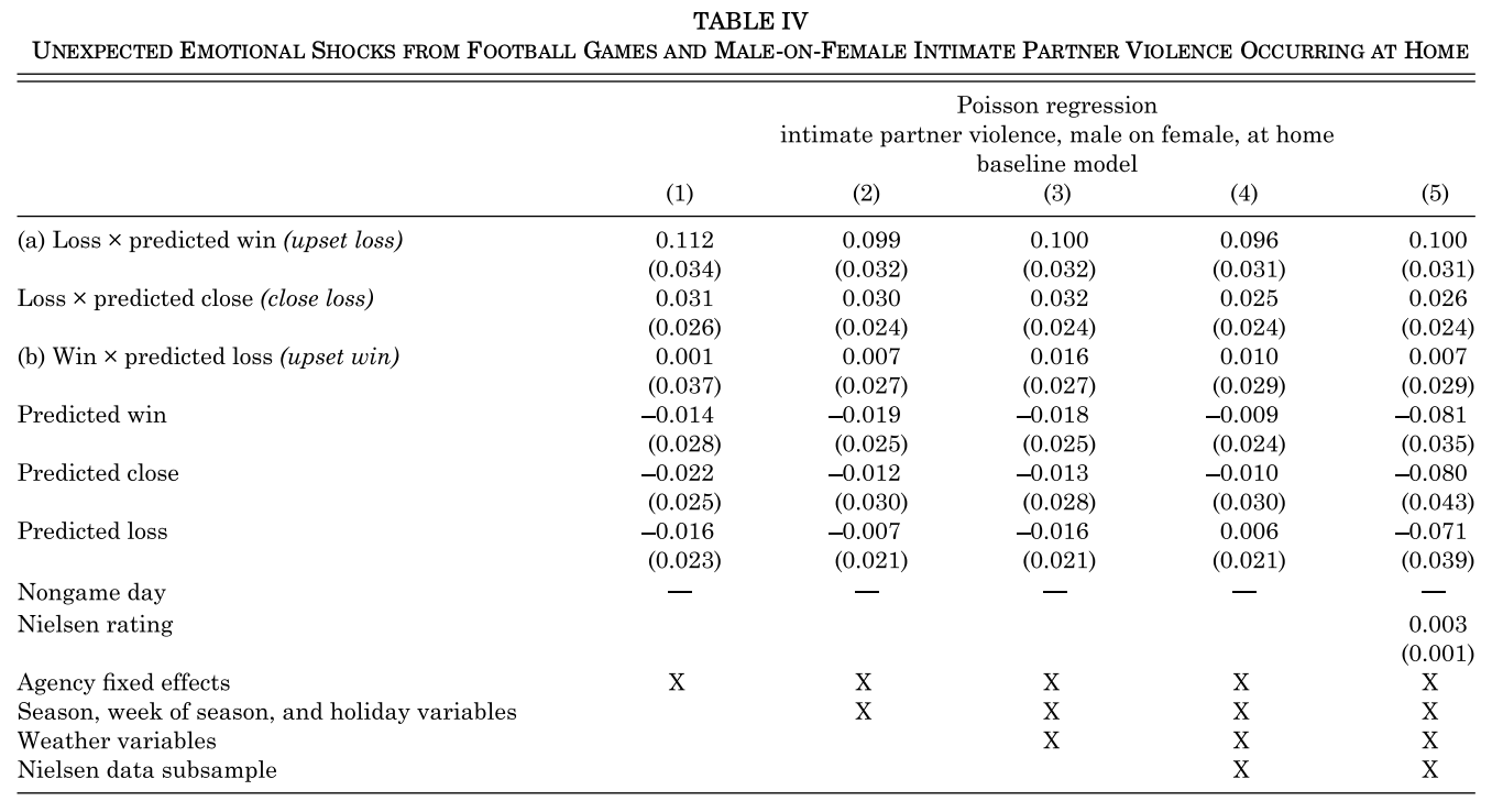
By comparing games with the same pre-game point spread, Card and Dahl (2011) isolate the emotional shock of an upset loss — a loss when your team was predicted to win.

An upset loss raises at-home male-on-female violence by about 10% — and it barely moves as more controls are added (columns 1→5). The summary control did the work.

Define “upset loss” carefully: not just losing, but losing when the market expected you to win — the emotional shock is the surprise. Then read the table across, left to right: the estimate barely budges as controls pile up. That stability is the evidence the summary control already absorbed the confounding. A number that refuses to move is a number you can start to trust.

Source: Card and Dahl (2011)

Do selective universities pay off?

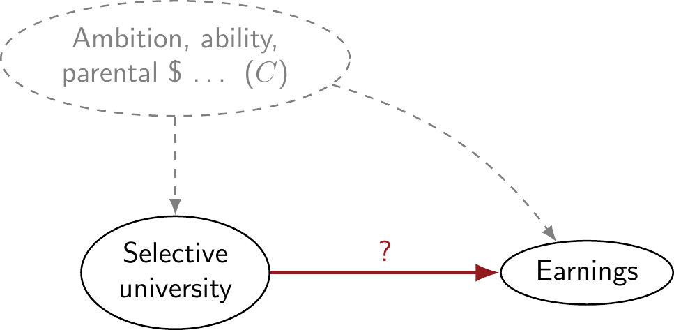
Graduates of selective universities earn more. But the ambitious, well-connected, and able both choose selective universities and earn more anyway — a swarm of confounders (\(C\)).

Discuss: what single thing could summarise a student’s ambition and ability as the admissions system saw it?

This one lands personally — they are all sitting in a selective university right now. Set up the problem honestly: graduates of selective schools do earn more, but the ambitious and able both choose those schools and would have earned more anyway. Let them chew on the blue box before the next slide; the answer is genuinely clever.

The smart summary control: where you applied

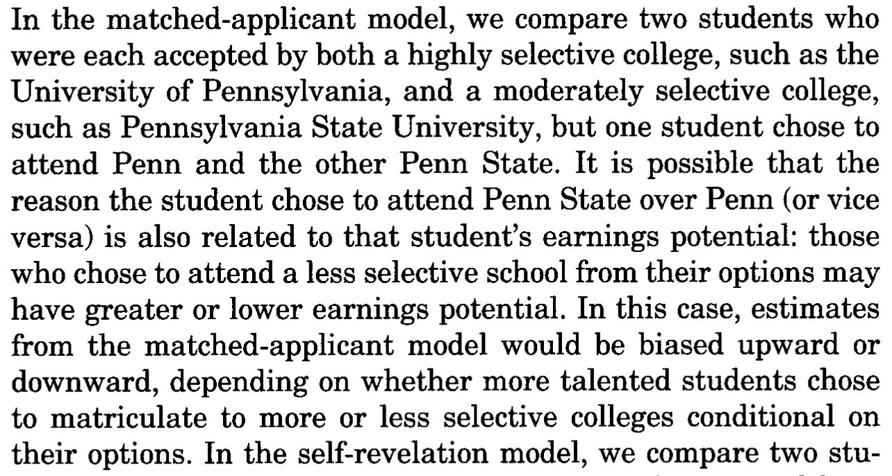
Dale and Krueger (2002) compare students who applied to and were admitted to the same set of schools — then some went to the more selective one, some did not.

Sharing an application portfolio is a summary of ambition and ability as the system measured it: a stand-in for the confounders no survey captures.

The insight: where you applied reveals how you saw yourself, and where you were admitted reveals how the system saw you. Two students with the same application portfolio and the same admissions letters are alike in ambition and ability without anyone ever measuring either. Then one enrolled at the selective school and the other did not — that is the comparison.

Source: Dale and Krueger (2002)

The premium disappears

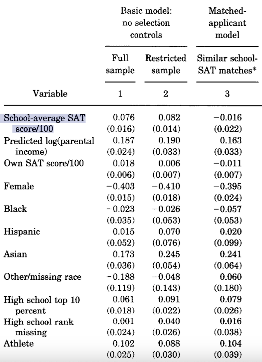
Without selection controls, each +100 points of school-average SAT buys about +7.6% earnings.

Among matched applicants, the effect collapses to −0.016 ≈ 0. The “selectivity premium” was mostly who chose selective schools, not the schools themselves.

+7.6% to essentially zero — pause on that. The premium was never the education; it was who walked through the door. Expect pushback, and welcome it: networks and signalling are real arguments. The honest reply is that this design tests the earnings premium for people who got in, and it does not survive.

Source: Dale and Krueger (2002)

No Harvard premium → no KU premium

If a selective US university barely raises earnings once you compare like with like, a selective Danish one probably doesn’t either.

\(\rightarrow\) Your KU degree pays off because you are able and put in the work — the diploma mostly reflects that, it does not manufacture it.

Deliver this as encouragement, not deflation: what pays off is the ability and the work, and the diploma mostly reports that back to employers. Worth naming the extrapolation as an extrapolation — this is US data, and Danish institutions differ. Good moment to ask what would make Denmark different.

Break

Your turn: exercise 2

You visualise the adjustment: a before/after coefficient plot and model predictions — again on the carbon divide.

Open exercise 2 in a new tab ↗

Today’s general lessons

1. A confounder opens a backdoor path (arrow into the treatment) — control it. A mediator lies on the causal path (arrow out of the treatment) — usually don’t, or you delete part of the effect.

2. Adding a control can move a coefficient a lot — even flip its sign (state ownership & poverty). Always ask why a variable belongs in the model.

3. Frisch–Waugh: “controlling for \(C\)” = residualise \(Y\) on \(C\), residualise \(D\) on \(C\), regress the residuals. Same number, clearer intuition.

4. When confounders are unmeasurable, a smart summary control — a point spread, a shared application portfolio — can stand in for many of them at once.

5. Multiple OLS improves comparisons; only a real experiment guarantees them.

Point five is the one to say slowly, because it is the whole course in one line: controlling makes a comparison fairer, never fair. You can only ever adjust for confounders you thought of and measured. That gap is exactly why the coming weeks look for natural experiments instead.

Check yourself: today’s goals

• Point to the confounder and the mediator on a DAG, and say which you would put in the regression — and why.
• Explain, in the three Frisch–Waugh steps, what “holding civil liberties constant” does to the state ownership coefficient.
• Give one example of a smart summary control and the confounders it stands in for.

Shaky on any of these? That is what this week’s Absalon quiz and the Friday exercise class are for.

Today’s important functions

• lm_robust(y ~ d + c, ...): multiple OLS — the coefficient on d holds c constant.
• modelr::add_residuals(model = ..., var = ...): keep a model’s residuals (the Frisch–Waugh workflow).
• tidy() + geom_pointrange() + coord_flip(): the coefficient plot.
• predict(model, newdata = ..., interval = "confidence"): predictions — set controls to an informative constant.
• modelsummary(list(...)): put bivariate and multiple models side by side.

References

Angrist, J. D. and J. Pischke (2014). Mastering ’Metrics: The Path from Cause to Effect. Princeton University Press.

Card, D. and G. B. Dahl (2011). “Family Violence and Football: The Effect of Unexpected Emotional Cues on Violent Behavior*“. In: The Quarterly Journal of Economics, pp. 103-143.

Dale, S. B. and A. B. Krueger (2002). “Estimating the Payoff to Attending a More Selective College: An Application of Selection on Observables and Unobservables*“. In: The Quarterly Journal of Economics, pp. 1491-1527.

Frisch, R. and F. V. Waugh (1933). “Partial Time Regressions as Compared with Individual Trends”. In: Econometrica, pp. 387-401.