Randomised Controlled Trials

The gold standard of causal inference

Merlin Schaeffer · Department of Sociology

2026-07-28

 

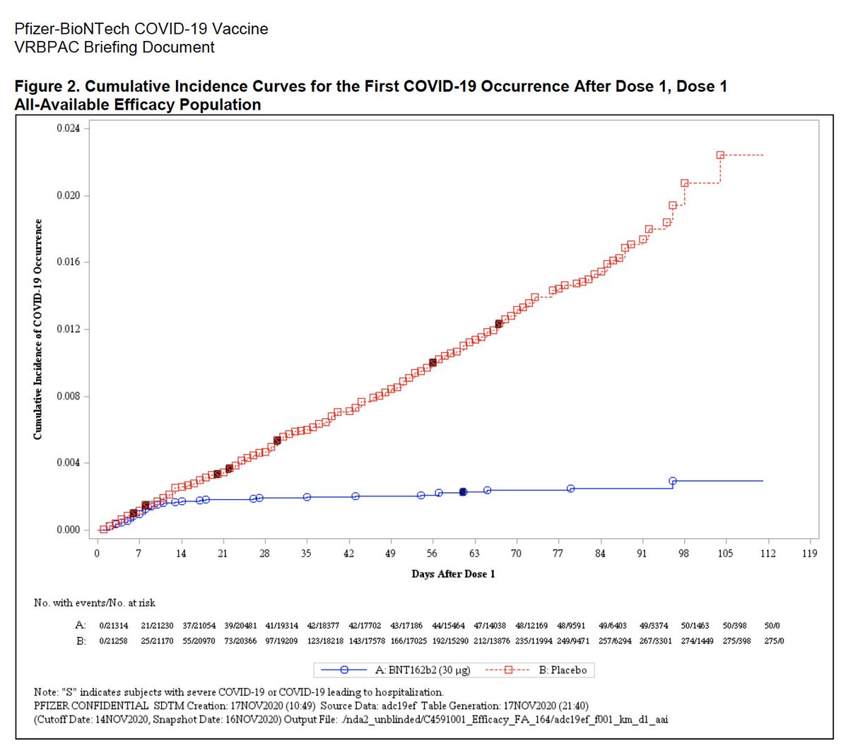
How do we know it works?

Source: Polack, Thomas, Kitchin, Absalon, Gurtman, Lockhart, Perez, Pérez Marc, Moreira, Zerbini, Bailey, Swanson, Roychoudhury, Koury, Li, Kalina, Cooper, Frenck, Hammitt, Türeci, Nell, Schaefer, Ünal, Tresnan, Mather, Dormitzer, Şahin, Jansen, and Gruber (2020)

Open with the question, not the answer: they all took this vaccine — how does anyone actually know it works? Let them try for a moment. The answer is the design, not the statistics: tens of thousands of people, a coin flip deciding who got the shot. That design is today’s whole lecture.

Goal of empirical sociology

Use data to discover patterns,
and the social mechanisms that bring them about.

By the end of today you can …

1. explain why a simple group comparison can mislead us — selection bias;

2. see how randomisation fixes it — in one picture and one formula;

3. estimate a causal effect from a real experiment in R.

One part of today’s lecture per goal. Our running question throughout: does news media consumption increase immigrant minorities’ reports of discrimination?

Three goals, three parts — say that explicitly so they can locate themselves later. Flag the arc: we start with a comparison that fails, then the one idea that repairs it, then they estimate a real causal effect themselves in R. Last week’s lecture diagnosed the disease; today is the cure.

The Integration Paradox

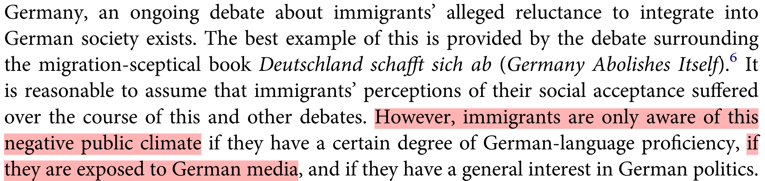
Immigrants who are better integrated — e.g. higher educated, fluent in the language — report more discrimination, not less.

One suspected channel: the news media (highlighted in the study on the right).

Research question of the day: does news media consumption increase immigrant minorities’ reports of discrimination?

Source: Steinmann (2019)

Remind them of the paradox from last week — better integrated, more reported discrimination. Today we chase one suspected channel: the news media. Put the research question on the board and leave it there; every slide today is in service of answering it.

Why naïve comparisons mislead

Part 1 of 3

Just comparing news-readers with non-readers will not give us a causal effect. Let’s see why.

Preparation

• Packages for today’s session
• The APAD survey
• Get the APAD data

pacman::p_load( # Load several R packages using the pacman package manager
  tidyverse,  # A collection of packages for data manipulation and visualization
  ggplot2,    # Powerful package for creating static, animated and interactive visualizations
  estimatr,   # Package for fast estimators for regression with weighted data
  modelr,     # Provides functions for modelling and prediction
  kableExtra, # Enhances table creation in R
  modelsummary) # Creates tables and plots to summarise statistical models

• Schaeffer, Kas, and Hagedorn (2023)
• 1093 immigrants and children of immigrants.
• Berlin, Hamburg, Munich, Frankfurt, Cologne.
• Interviewed August 2021.
• Financed by the German Research Council (DFG)

1. On a typical day, about how much time do you spend watching, reading, or listening to news about politics and current affairs? Please give your answer in hours and then minutes.

2. How often were you personally discriminated against in the following situations here in Germany? Discrimination means a person is treated worse than others, with no factual justification — e.g. insult, ostracism, harassment. Disadvantaging rules and laws also count. … looking for work  ·  at work  ·  in education
   … looking for housing  ·  with officials  ·  in public
   
   

   1. Never (2) Rarely (3) Sometimes (4) Often (5) Very often

load("APAD.RData") # Load APAD dataset

APAD <- APAD %>% # Process the APAD data
  mutate(
    # News consumption in minutes (e.g. 2h 30m -> 150)
    news = news_hrs * 60 + news_mins,
    # Binary: reads >= 15 minutes of news per day?
    news_yn = case_when(
      news <  15 ~ 0,
      news >= 15 ~ 1,
      TRUE       ~ as.numeric(NA)
    ),
    # Average perceived discrimination across 6 domains
    dis_index = rowMeans(
      select(., dis_trainee, dis_job, dis_school,
             dis_house, dis_gov, dis_public),
      na.rm = TRUE
    ),
    # z-standardised version (mean 0, SD 1)
    z_dis_index = scale(dis_index) %>% as.numeric()
  )

# # A tibble: 1,093 × 24
#    antidiscr_law dis_index news_hrs news_mins dis_trainee dis_job dis_school dis_house dis_gov dis_public gewFAKT
#            <dbl>     <dbl>    <dbl>     <dbl>       <dbl>   <dbl>      <dbl>     <dbl>   <dbl>      <dbl>   <dbl>
#  1             5      3.17        1         0           3       3          4         5       2          2   0.105
#  2             4      1.8         1         1           5      NA          1         1       1          1   0.103
#  3             3      2           0        30           1       2          1         3       3          2   0.802
#  4             5      2.83        0        10           3       3          2         5       1          3   0.104
#  5             4      3.2         0        30           2       3         NA         5       3          3   0.639
#  6             5      2.75        2         0          NA       2         NA         4       3          2   0.2  
#  7             2      1           3        58           1       1          1         1       1          1   2.42 
#  8             4      1.67        5         0           3       1          1         3       1          1   0.102
#  9             5      4           1        15           4       4          4         4       4          4   6.19 
# 10             4      1.33        0        30           1       2          1         1       1          2   2.08 
# # ℹ 1,083 more rows
# # ℹ 13 more variables: gender <fct>, age <dbl>, imor <fct>, german <fct>, nbh_exposed <dbl>, appearance <fct>,
# #   article <chr>, ment_happy <dbl>, leftright <dbl>, gen_trust <dbl>, news <dbl>, news_yn <dbl>,
# #   z_dis_index <dbl>

Naïve comparison

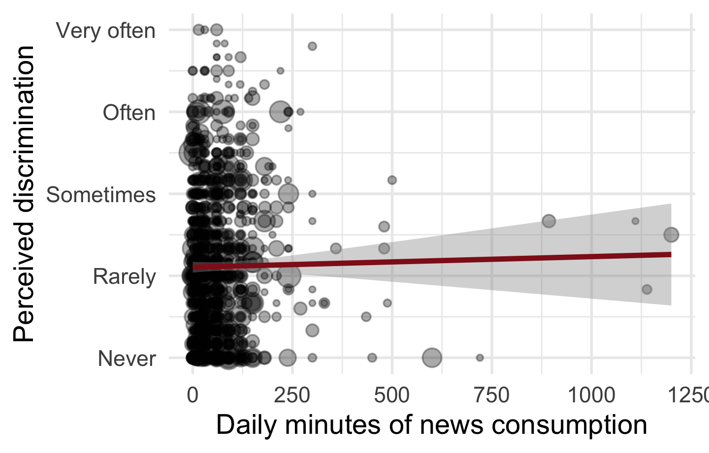
Discuss: we find a tiny association. Can we trust it as the effect of news?

No — news-readers and non-readers differ in many other ways.

Ask before revealing: we found a tiny association — can we read it as the effect of news? Most will hesitate, which is the right instinct. The reveal names why: readers and non-readers differ in many other ways, so we are not comparing like with like. Do not over-explain here — the next three slides do the work.

ols <- lm_robust( # Weighted OLS
  dis_index ~ news_yn,
  weights = gewFAKT,
  data = APAD
)

modelsummary( # Regression table
  list("Discr." = ols),             # Named list of models
  stars = TRUE,                     # Significance stars
  gof_map = c("nobs", "r.squared"), # Fit statistics to show
  output = "kableExtra"
)

	Discr.
(Intercept)	2.187***
	(0.116)
news_yn	−0.093
	(0.129)
Num.Obs.	1085
R2	0.002
+ p < 0.1, * p < 0.05, ** p < 0.01, *** p < 0.001

The dream: two parallel worlds

To know the causal effect, we’d compare the same person — reading news vs. not.

Person	If reads news (\(Y_1\))	If no news (\(Y_0\))	Causal effect
Aisha	4	?	?
Ben	?	2	?
Chen	5	?	?

Discuss: what would we need in order to measure one person’s causal effect?

Both worlds at once — impossible. The missing cell is the counterfactual: the fundamental problem of causal inference.

Point at the grey question marks — one per person, always exactly one. Ask what we would need to measure a single person’s causal effect, and let them arrive at the impossible answer: both worlds at once. Name it once, clearly: the missing cell is the counterfactual, and this is the fundamental problem of causal inference.

Why the naïve comparison misleads

The raw gap between readers and non-readers mixes two things:

\[ \underbrace{Avg_{n}[Y_{1i}|D_{i}=1] - Avg_{n}[Y_{0i}|D_{i}=0]}_{\text{Difference we actually observe}} = \underbrace{\color{#901A1E}{\kappa}}_{\substack{\text{causal}\\\text{effect}}} + \underbrace{Avg_{n}[Y_{0i}|D_{i}=1] - Avg_{n}[Y_{0i}|D_{i}=0]}_{\text{selection bias}} \]

Discuss: which term do we actually want — and which one gets in the way?

We want the causal effect \(\color{#901A1E}{\kappa}\). Selection bias is the contamination: the groups already differed in baseline \(Y_0\), before any news.

Do not read the formula symbol by symbol — point at the two braces instead. What we observe is one number; it silently contains two things. Ask which one they want and which one is in the way, then reveal. The phrase to repeat all day: the groups already differed before any news.

Do the groups actually differ?

• Balance table
• R code

Discuss: do news-readers and non-readers look the same on their background traits?

Who reads the news? Background of readers vs non-readers

		0		1
		Mean	Std. Dev.	Mean	Std. Dev.	Diff. in Means	Std. Error
age		36.7	12.3	43.8	15.4	7.1	2.2
nbh_exposed		4.2	0.8	4.2	1.0	−0.0	0.1
		N	Pct.	N	Pct.
imor	Child of immigrant	64	29.4	399	45.6
	Immigrant	154	70.6	476	54.4
german	Ja	89	40.8	561	64.1
	Nein	129	59.2	314	35.9

No — readers are older and more often German citizens. The comparison is confounded.

Let them inspect the columns before you reveal — ask them to find the biggest gap. Age and citizenship jump out. This is the abstract selection-bias term made visible in an actual table, so say so: this is what contamination looks like in data. And add the caveat — these are only the variables we happened to measure.

APAD %>% # Start with the APAD data, then pipe
  # Compare readers vs non-readers on background variables
  select(news_yn, age, nbh_exposed, imor, german, gewFAKT) %>%
  # datasummary_balance() treats a column called `weights` as survey weights
  rename(weights = gewFAKT) %>%
  datasummary_balance(
    formula = ~ news_yn, # Split the table by news_yn (0 vs 1)
    data = .,
    title = "Who reads the news? Background of readers vs non-readers",
    output = "kableExtra"
  )

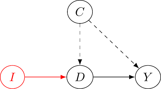
Seeing the problem: a DAG

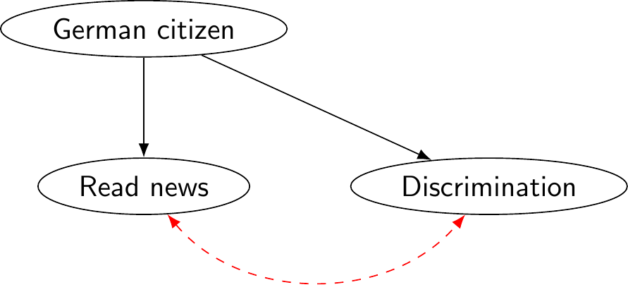
Reading a DAG: an arrow means “causes”.

Discuss: the red link is a correlation. Why is it not a causal effect?

Citizenship drives both news use and discrimination → it opens a backdoor path. The link is spurious.

Same picture they met last week, so keep it quick. Trace the red link and ask why it is not a causal effect. The reveal: citizenship feeds both boxes, which opens a backdoor path — correlation flows along it without any causal arrow between news and discrimination.

The fix: experiments & randomisation

Part 2 of 3

If observing can’t tell us, we intervene — and let a coin decide who gets the treatment.

Experiment: we don’t watch, we act

• We don’t passively observe — we actively intervene.

• We decide who gets the treatment \(D\) and who doesn’t.

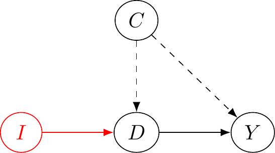
Discuss: how can our intervention \(\color{red}{I}\) cut the link between treatment \(D\) and confounders \(C\)?

The pivot of the lecture: we stop watching and start acting. We decide who gets the treatment, which means the confounders no longer get to. Pose the question and let them sit with it over the break — the answer is the next part.

Break

 

Open exercise 1 in a new tab ↗

Break

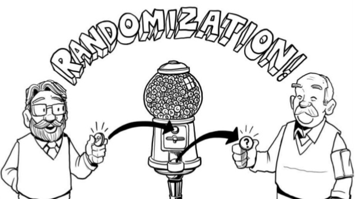
Randomised Controlled Trial (RCT)

We flip a coin — randomly deciding who gets the treatment:

• \(\text{News} = 0 \rightarrow\) Control group
• \(\text{News} = 1 \rightarrow\) Treatment group

Because assignment is random, it can not be driven by citizenship, age, or anything else.

Define the RCT plainly: a coin, not a person and not a preference, decides who is treated. The consequence is the sentence in the green box — assignment cannot be driven by citizenship, age, or anything else, because a coin knows none of those things.

Why randomisation works: a fair coin

A fair coin gives everyone the same chance of treatment, regardless of who they are.

So the two groups look alike on average — on age, citizenship, and on things we can’t even measure.

Equal baselines:
\(Avg_{n}[Y_{0i}|\text{News}=1] = Avg_{n}[Y_{0i}|\text{News}=0]\)

This is the single most important idea of the course, so slow down. A fair coin gives everyone the same chance of treatment regardless of who they are — so the two groups end up alike on age, on citizenship, and on everything we never thought to measure. That last clause is what no amount of statistical adjustment can buy you.

Why it works: the selection bias vanishes

Randomly split subjects → both groups come from the same underlying population.

\(\rightarrow\) similar on average in every way, including their baseline \(Y_0\).

\(\rightarrow\) so \(E[Y_{0i}|D=1] = E[Y_{0i}|D=0]\), and selection bias = 0.

Beware: randomisation can still fail by chance — especially in small samples.

\[ \begin{aligned} & E[Y_{1i}|D=1] - E[Y_{0i}|D=0] \\[4pt] & = E[Y_{0i} + \color{#901A1E}{\kappa}\,|D=1] - E[Y_{0i}|D=0] \\[4pt] & = \color{#901A1E}{\kappa} + \underbrace{E[Y_{0i}|D=1] - E[Y_{0i}|D=0]}_{= \; 0 \;\text{ if randomised}} \\[4pt] & = \underbrace{\color{#901A1E}{\kappa}}_{\text{the average causal effect}} \end{aligned} \]

Walk the four lines slowly — it is the same decomposition as before, but now one term dies. Randomisation makes the baselines equal, so selection bias is zero and what remains is the causal effect. Do not skip the red box: randomisation can still fail by chance, especially in small samples, which is exactly why we run a balance test afterwards.

Why it works: no backdoor in the DAG

Randomising \(I\) means no arrow points into it.

\(\Rightarrow\) no backdoor path from \(I\) to \(Y\).

\(\Rightarrow\) no confounding, no selection bias.

The same result in pictures for the students who don’t think in algebra. The point to make with your finger: nothing points into the red node, because we control it. No incoming arrow means no backdoor path, which means no confounding. Formula people and picture people should both leave convinced.

A real experiment, in R

Part 3 of 3

We ran an actual RCT inside the APAD survey — now we estimate its causal effect ourselves.

 

The APAD survey experiment

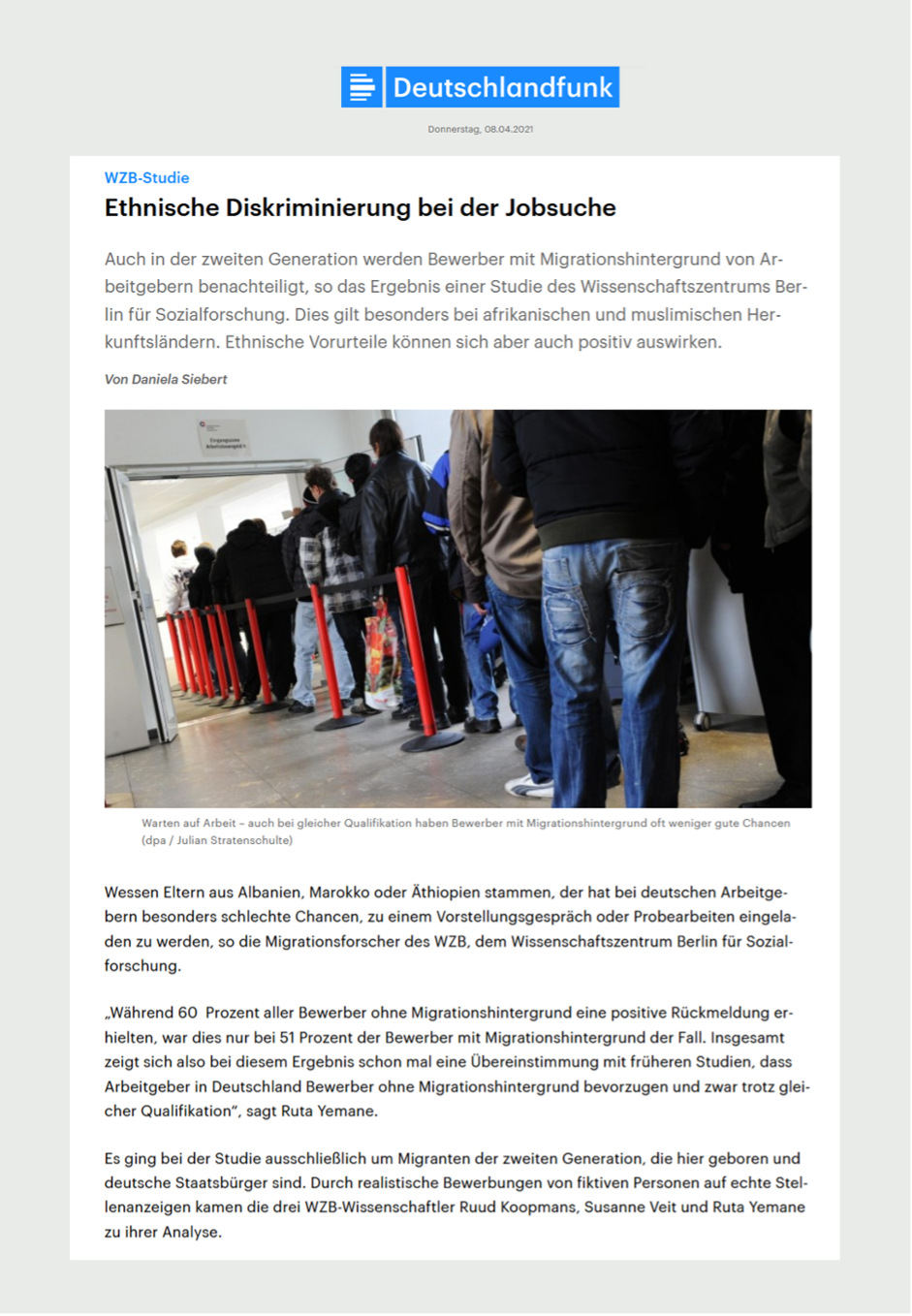
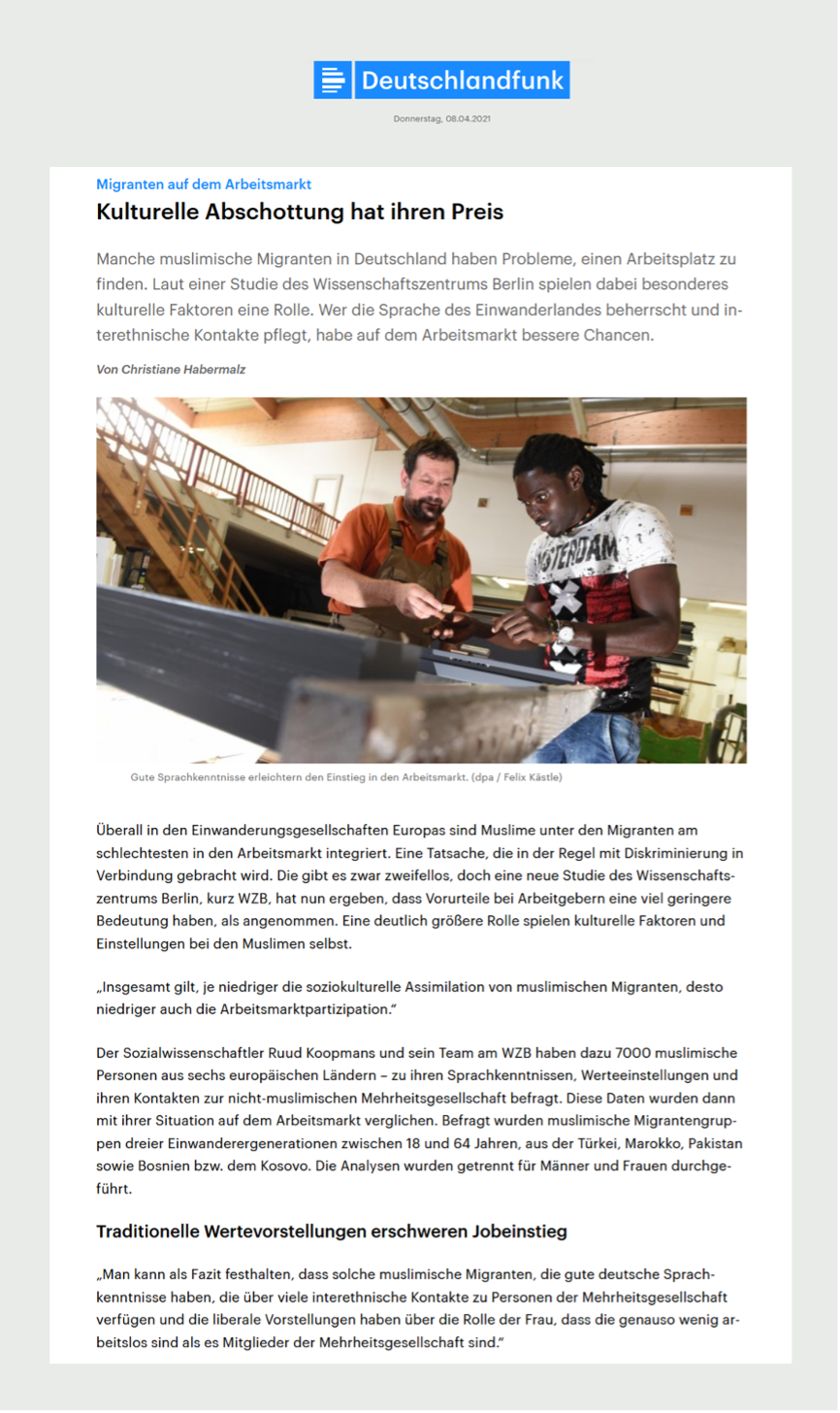
We asked subjects to read a news article — and randomly decided which one:

• Venus \(\rightarrow\) Control group
• Discrimination \(\rightarrow\) Treatment 1
• Acculturation \(\rightarrow\) Treatment 2

Now it stops being hypothetical: we built an experiment inside the survey they already know. Everyone read an article; a random draw decided which one — Venus for the control, discrimination or acculturation for the two treatments. Stress that respondents could not choose, and did not know there was a draw.

 

 

Did randomisation balance the groups?

• Surveyed news reading
• Randomised article
• R code

Who reads the news? Background of readers vs non-readers

		0		1
		Mean	Std. Dev.	Mean	Std. Dev.	Diff. in Means	Std. Error
age		36.7	12.3	43.8	15.4	7.1	2.2
nbh_exposed		4.2	0.8	4.2	1.0	−0.0	0.1
		N	Pct.	N	Pct.
imor	Child of immigrant	64	29.4	399	45.6
	Immigrant	154	70.6	476	54.4
german	Ja	89	40.8	561	64.1
	Nein	129	59.2	314	35.9

Beware: the observational split is imbalanced — the groups differed before any treatment.

Background of the randomly assigned treatment groups

		Contr (N=358)		Treat_1 (N=375)		Treat_2 (N=360)
		Mean	Std. Dev.	Mean	Std. Dev.	Mean	Std. Dev.
news_yn		0.8	0.4	0.8	0.4	0.8	0.4
age		41.8	15.7	41.2	12.4	43.8	16.9
nbh_exposed		4.2	0.9	4.2	1.1	4.2	1.0
		N	Pct.	N	Pct.	N	Pct.
imor	Child of immigrant	156	43.6	157	41.9	150	41.7
	Immigrant	202	56.4	218	58.1	210	58.3
german	Ja	215	60.1	222	59.2	213	59.2
	Nein	143	39.9	153	40.8	147	40.8

Randomised split: the groups are balanced — exactly what randomisation buys us.

This pair of tabs is the payoff of the whole lecture, so put them side by side deliberately. Same data, same background variables, two different ways of splitting people: the surveyed split is imbalanced, the randomised split is balanced. Nothing about the respondents changed — only who decided. That contrast is worth a full minute of silence.

APAD %>% # Start with the APAD data, then pipe
  # Keep the treatment indicator, background variables, and survey weights
  select(article, news_yn, age, nbh_exposed, imor, german, gewFAKT) %>%
  # datasummary_balance() treats a column called `weights` as survey weights
  rename(weights = gewFAKT) %>%
  datasummary_balance(
    formula = ~ article, # Split the table by the randomised treatment
    data = .,
    title = "Background of the randomly assigned treatment groups",
    output = "kableExtra"
  )

The causal effect

# Weighted OLS on the survey experiment
ols  <- lm_robust(dis_index ~ article, weights = gewFAKT, data = APAD)

# Same, but on the z-standardised outcome (effect in SDs)
zols <- lm_robust(z_dis_index ~ article, weights = gewFAKT, data = APAD)

modelsummary( # Regression table with readable labels
  list("Discr." = ols, "Z-Discr." = zols),
  stars = TRUE,
  coef_map = c(
    "(Intercept)"    = "Intercept (Venus control)",
    "articleTreat_1" = "Article on discrimination",
    "articleTreat_2" = "Article on acculturation"
  ),
  gof_map = c("nobs", "r.squared"),
  output = "kableExtra"
)

	Discr.	Z-Discr.
Intercept (Venus control)	1.979***	−0.171*
	(0.067)	(0.074)
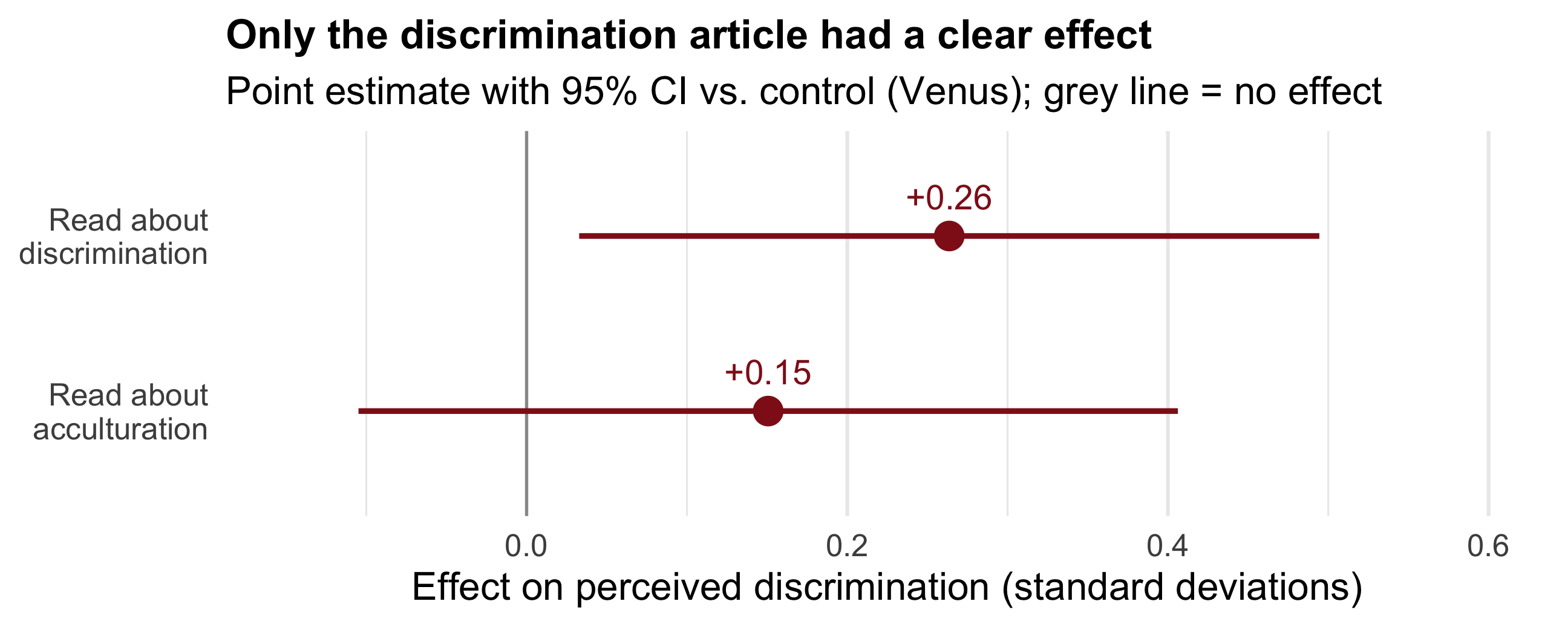
Article on discrimination	0.239*	0.264*
	(0.107)	(0.118)
Article on acculturation	0.137	0.151
	(0.118)	(0.130)
Num.Obs.	1085	1085
R2	0.012	0.012
+ p < 0.1, * p < 0.05, ** p < 0.01, *** p < 0.001

Because assignment was random, this difference is the causal effect \(\kappa\) — no confounding to worry about.

Note how ordinary the code is — it is the same lm_robust() they have run for weeks. That is the lesson: the credibility came from the design, not from a fancier estimator. Read the discrimination-article coefficient aloud, then say the sentence they should be able to repeat: because assignment was random, this difference is the causal effect.

Visualise the effect

• Plot
• R code

plotdata <- zols %>%
  tidy() %>%                        # Coefficients as a tibble
  filter(term != "(Intercept)") %>% # Keep only the treatment effects
  mutate(term = recode(
    term,
    "articleTreat_1" = "Read about\ndiscrimination",
    "articleTreat_2" = "Read about\nacculturation"
  ))

ggplot(plotdata, aes(x = estimate, y = term)) +
  geom_vline(xintercept = 0, linewidth = 0.6, colour = "grey60") +
  geom_pointrange(aes(xmin = conf.low, xmax = conf.high),
                  colour = "#901A1E", linewidth = 1.1, size = 1) +
  geom_text(aes(label = sprintf("%+.2f", estimate)),
            vjust = -1.1, size = 5, colour = "#901A1E") +
  scale_x_continuous(limits = c(-0.15, 0.6)) +
  labs(x = "Effect on perceived discrimination (standard deviations)", y = NULL,
       title = "Only the discrimination article had a clear effect",
       subtitle = "Point estimate with 95% CI vs. control (Venus); grey line = no effect") +
  theme_minimal(base_size = 16) +
  theme(panel.grid.major.y = element_blank(),
        plot.title = element_text(face = "bold", size = rel(1.05)))

Read the plot as a picture first: the grey line is “no effect”, and a whole interval sitting clear of it is what a real finding looks like. Only the discrimination article moved people; acculturation did essentially nothing. Ask them what a bar crossing the grey line would have meant — good check of last week’s inference.

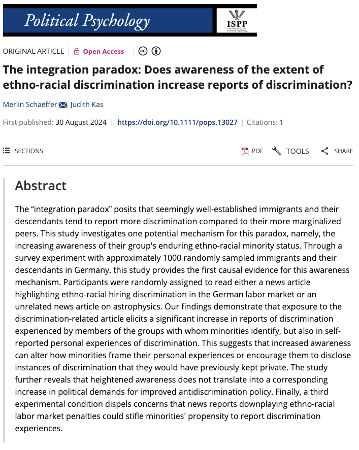
It’s real research!

Source: Schaeffer and Kas (2024)

Effects of experimentally induced awareness of discrimination

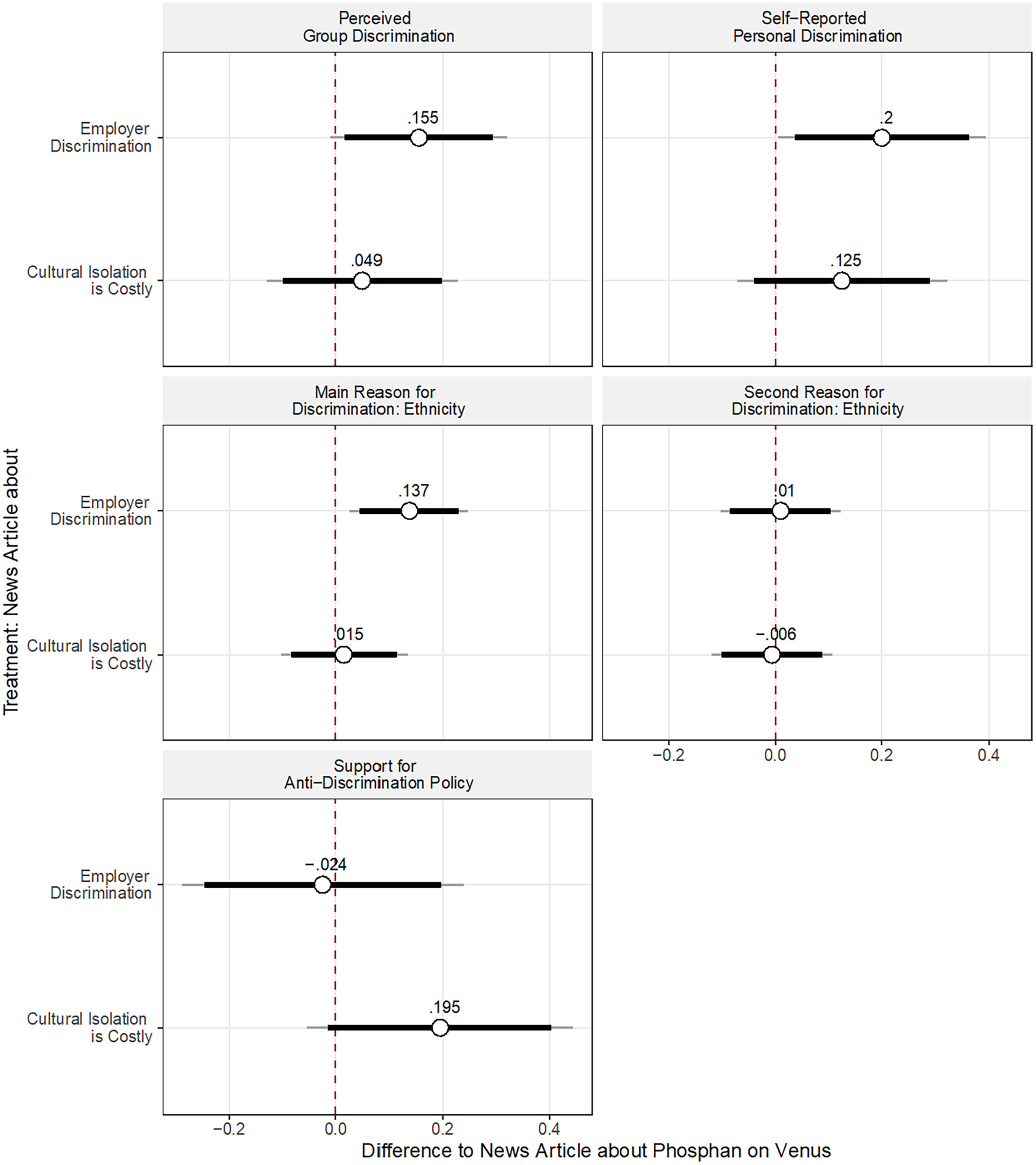
Point estimates with 90% and 95% confidence intervals, post-stratification-weighted OLS with (cluster-)robust standard errors.

Worth saying out loud: what they just estimated in class is a published paper, not a teaching toy. Their coefficient is in that figure. This is also the moment to mention that they will replicate this study themselves — it makes the exercise feel like research rather than homework.

 

Open exercise 2 in a new tab ↗

The logic in one line

• Experiment: we set the treatment, then watch the outcome.
• RCT: treatment assigned by chance → groups alike on everything, even the unmeasured.
• Balance test: our check that randomisation worked.
• OLS on an RCT: the coefficient is the causal effect.

Trace the chain left to right — it is the whole lecture in four boxes. “Randomise” is red because it is the only step that is a choice we make; everything downstream follows from it. If they remember one picture from today, this is the one.

But what if you can’t randomise?

Most of sociology can’t run experiments.

Then we try to make groups comparable after the fact — by statistically holding confounders constant.

That tool is multiple OLS regression — the heart of the next weeks.

End on the honest limitation. We cannot randomise someone’s citizenship, their neighbourhood, or their education — which rules out experiments for most of the questions sociologists actually care about. So the next weeks ask: can we make groups comparable after the fact? That is multiple regression, and it is a weaker tool than a coin — say that plainly now so they are properly sceptical later.

Check yourself: today’s goals

Look back at the goals from the start of the lecture. Can you tick all three?

• Explain selection bias to a friend in one sentence — why can a raw group comparison mislead?
• Show — with the DAG or the formula — why randomisation removes it.
• Run lm_robust() on an experiment in R and read the coefficient as a causal effect.

Anything feel shaky? That is what this week’s Absalon quiz and the Friday exercise class are for.

Today’s important functions

• estimatr::lm_robust(y ~ d, weights = ...): the RCT effect — a bivariate OLS of the outcome on the randomly assigned treatment (survey-weighted here).
• modelsummary::datasummary_balance(~ d, data = ...): the balance table — check treatment and control look alike on background traits (the payoff of randomisation).
• modelsummary(list("Model" = ...), stars = TRUE): a clean regression table.
• rowMeans(across(...)): average several survey items into one index.

References

Polack, F. P., S. J. Thomas, N. Kitchin, et al. (2020). “Safety and Efficacy of the BNT162b2 mRNA Covid-19 Vaccine”. In: New England Journal of Medicine, pp. 2603-2615.

Schaeffer, M. and J. Kas (2024). “The integration paradox: Does awareness of the extent of ethno-racial discrimination increase reports of discrimination?” In: Political Psychology.

Schaeffer, M., J. Kas, and P. Hagedorn (2023). “The Association between Actual and Perceived Discrimination (APAD): Technical Report”. In: SocArXiv.

Steinmann, J. (2019). “The paradox of integration: why do higher educated new immigrants perceive more discrimination in Germany?” In: Journal of Ethnic and Migration Studies, pp. 1377-1400.