Selection Bias

Why correlation ≠ causation — potential outcomes & confounding

Friedolin Merhout & Merlin Schaeffer · Department of Sociology

2026-07-23

By the end of today you can …

1. state a causal hypothesis as a counterfactual comparison — the potential-outcomes framework;

2. explain why a naïve comparison of two groups is usually not the causal effect — selection bias;

3. read a DAG — spot a confounder on a backdoor path — and use a balance test to expose it.

One part per goal. Our running question: does consuming news make immigrant minorities report more discrimination?

Frame the day: our goal is not describing patterns but explaining them — and today is about avoiding false explanations. Walk the arc once: a real-world puzzle, then a simple but flawed analysis, then the theory that fixes it (potential outcomes), then the tool that draws it (DAGs).

From hypothesis to comparison

Part 1 of 3

Every causal claim is secretly a comparison — of what happened against what would have happened.

The research question of the day

The integration paradox: immigrants and their descendants who are better integrated — more educated, longer resident — often report more discrimination, not less Schaeffer and Kas (2024).

One proposed mechanism: the better integrated consume more news, become more aware of discrimination, and so report it more often.

Research question: does consuming news increase how often immigrant minorities report discrimination?

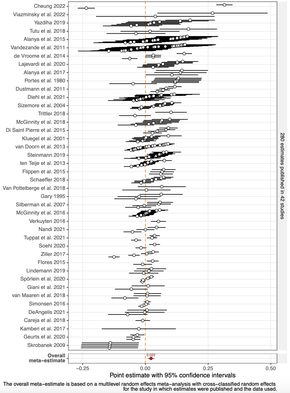
280 estimates from 42 studies; overall ≈ +0.022. Source: Schaeffer and Kas (2024)

Say the paradox out loud, because it is genuinely counterintuitive: the better integrated report more discrimination, not less. Point at the forest plot — 280 estimates from 42 studies, so this is a robust pattern, not one odd survey. Today we test one proposed mechanism: awareness, via news consumption.

A hypothesis is a comparison

A causal claim implies a counterfactual: things would have been different had \(X\) (not) happened.

\(H_1:\) news consumption increases how often minorities report discrimination:

\[0 < \text{Avg}_n[\text{Discr.} \mid \text{news} = 1] - \text{Avg}_n[\text{Discr.} \mid \text{news} = 0]\]

\(H_0:\) news consumption does not change it: the difference of the two group averages is \(\leq 0\).

Discuss: what comparison is implied by each classic claim? Marx — capitalist labour alienates people and reduces mental health. Simmel — city life increases nervous stimulation and makes residents distant.

The key idea: testing a hypothesis always implies a comparison — causality is a counterfactual, a “what if”. Give them two minutes on Marx and Simmel, then collect: Marx compares capitalist against non-capitalist labour, Simmel urban against rural life. Every causal claim names two worlds, even when it doesn’t say so.

Why not just ask people?

The obvious “study”: ask people “How does reading the news affect you?”

Discuss: why is simply asking a bad way to test our hypothesis?

People have inaccurate perceptions of what shapes them — social desirability, faulty memory, little self-insight. Statements by research subjects are valuable, but they are not credible causal evidence. We need a comparison, not an introspection.

Ask first — give them two minutes before you click the reveal. Expect: social desirability, poor memory, lack of self-awareness. The line to land: people tell interesting stories about their lives, they do not record causal facts about themselves. So we need a comparison, not an introspection.

Preparation

• Packages
• The APAD survey
• Get & prepare the data

pacman::p_load(
  tidyverse,    # Data manipulation and visualization
  estimatr,     # OLS with robust / weighted standard errors
  modelsummary  # Regression AND balance tables
)

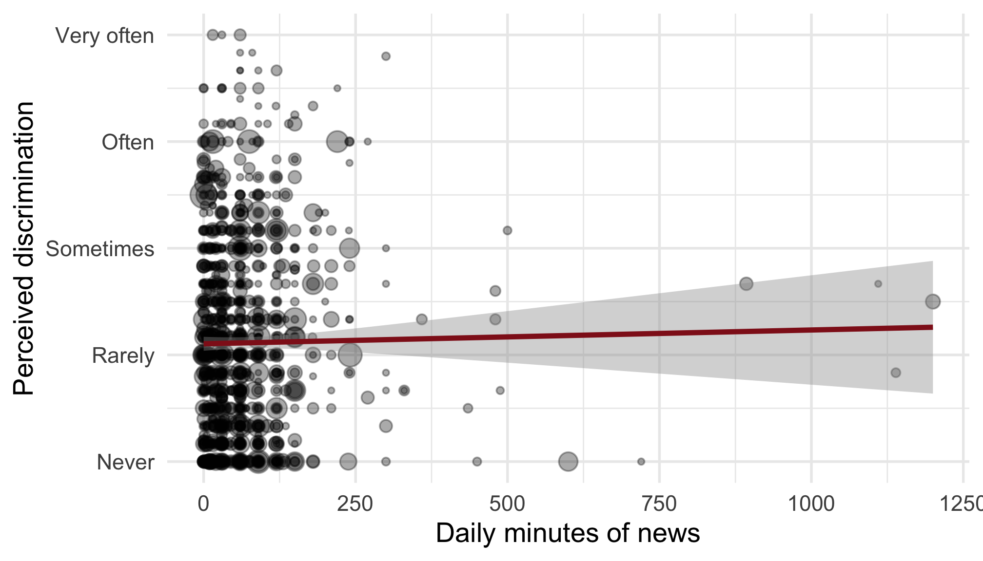
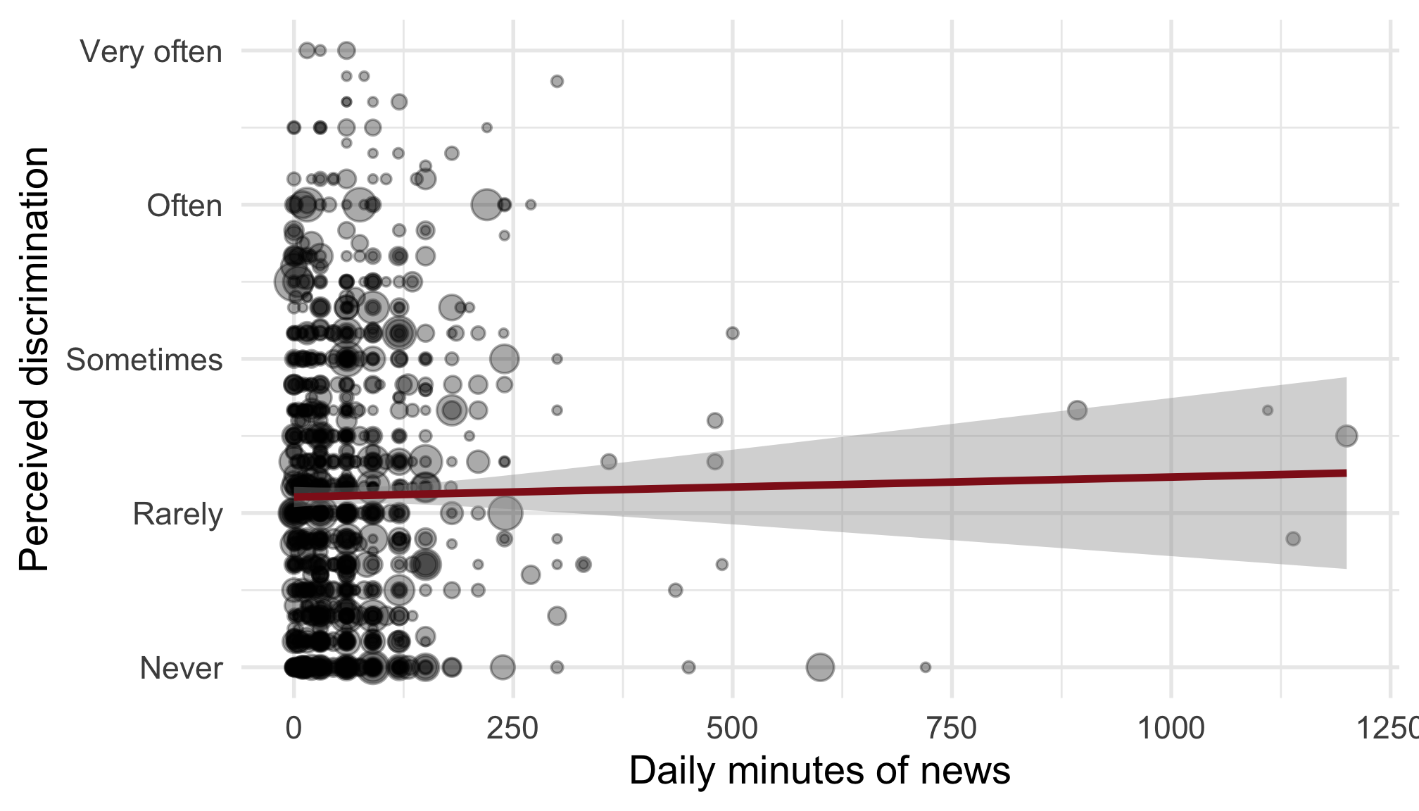
Schaeffer, Kas, and Hagedorn (2023) — 1,093 immigrants and children of immigrants in Berlin, Hamburg, Munich, Frankfurt & Cologne, interviewed August 2021.

1. “On a typical day, about how much time do you spend watching, reading, or listening to news about politics and current affairs?” (hours + minutes)

2. “How often were you personally discriminated …” — when looking for work, at work, in education, looking for housing, with officials, out in public. (1) Never … (5) Very often — averaged into one index.

# APAD ships as a local file (download it from Absalon into your project folder)
load("../assets/APAD.RData")

APAD <- APAD %>%
  mutate(
    news    = news_hrs * 60 + news_mins,          # total daily minutes
    news_yn = if_else(news >= 15, 1, 0),          # reads news? (>= 15 min)
    dis_index = rowMeans(                          # average across the 6 domains
      select(., dis_trainee, dis_job, dis_school,
             dis_house, dis_gov, dis_public),
      na.rm = TRUE
    )
  )

Keep this short — it is scaffolding, not the point. Two things only: the outcome dis_index averages the six discrimination domains into one index, and the cause comes in two forms, total daily minutes and a “reads news” dummy at 15 minutes. Then move on; the payoff is the next slide.

The naïve comparison

• The picture
• The regression
• Read it

# Weighted OLS: discrimination on the news dummy
ols <- lm_robust(dis_index ~ news_yn, weights = gewFAKT, data = APAD)

modelsummary(list("Discrimination" = ols), stars = TRUE,
             coef_rename = c("news_yn" = "Reads news"),
             gof_map = c("nobs", "r.squared"), output = "kableExtra")

	Discrimination
(Intercept)	2.187***
	(0.116)
Reads news	−0.093
	(0.129)
Num.Obs.	1085
R2	0.002
+ p < 0.1, * p < 0.05, ** p < 0.01, *** p < 0.001

News readers report, if anything, 0.09 points less discrimination — and the difference is not significant (\(t \approx -0.7\)). Taken at face value, \(H_1\) looks wrong. But is this a fair comparison?

Ask them to interpret the scatter before you show the table — two minutes with a neighbour. The line is flat, if anything slightly negative, so visually it does not support our hypothesis. Then the regression: about −0.09, not significant. Let them draw the obvious conclusion that the hypothesis is wrong — and then ask whether this is a fair comparison. That question is the rest of the lecture.

Break

Your turn: exercise 1

You run the naïve analysis yourself — on a different outcome: support for an anti-discrimination law.

Open exercise 1 in a new tab ↗

Potential outcomes & selection bias

Part 2 of 3

To see why the comparison can mislead, we need the language of potential outcomes.

Two futures for one person

For Ferda, two potential outcomes — one for each version of her life:

\[\text{effect}_{\text{Ferda}} = Y_{1,\text{Ferda}} - Y_{0,\text{Ferda}}\]

Ferda
\(Y_0\): discrimination without news	2 (rarely)
\(Y_1\): discrimination with news	4 (often)
Personal causal effect	+2

The fundamental problem of causal inference: we only ever see one of Ferda’s two futures. The other potential outcome is always missing — so a personal causal effect can never be observed directly.

Ferda makes it concrete: 4 with news, 2 without, so her personal causal effect is +2. Now the hard part — in reality we see only one of those two rows; the other is gone forever. That is the fundamental problem of causal inference, and it is exactly why we cannot fix this by asking people to imagine the other path.

The average causal effect

\[\text{Avg}_n[Y_{1i} - Y_{0i}] = \frac{1}{n}\sum_{i=1}^{n} Y_{1i} - \frac{1}{n}\sum_{i=1}^{n} Y_{0i}\]

The average causal effect is just the average of everyone’s personal causal effects.

It compares two whole worlds: one where everyone reads the news, against one where no one does. Neither world is ever fully observed — but, under the right conditions, we can estimate the average.

We give up on personal effects and aim for the average instead. Conceptually it compares two whole worlds — everyone reads the news, nobody does — and neither is ever observed. But the average is estimable under the right conditions, and what those conditions are is essentially the rest of this course.

Apples and oranges: Ferda vs. Tuki

We can’t see Ferda’s missing future — so what if we compare her to Tuki, who doesn’t read news?

	Ferda	Tuki
\(Y_0\): without news	2	5
\(Y_1\): with news	4	5
true effect	+2	0

Grey = the counterfactual we never see.

\[\underbrace{Y_{1,\text{Ferda}}}_{4} - \underbrace{Y_{0,\text{Tuki}}}_{5} = -1\]

Discuss: Ferda’s true effect is \(+2\), yet comparing her to Tuki gives \(-1\). Why is comparing different people so misleading here?

Since we cannot see Ferda’s missing future, we substitute a different person — that is what every observational comparison does. The result is −1, a terrible estimate of either person’s true effect. Give them two minutes on “why is this so wrong?”; the answer you are steering to is that they were different people to begin with.

The hidden term: selection bias

\[\underbrace{Y_{1,\text{Ferda}}}_{4} - \underbrace{Y_{0,\text{Tuki}}}_{5} = \underbrace{Y_{1,\text{Ferda}} - Y_{0,\text{Ferda}}}_{\text{true effect: }4-2 = +2} + \underbrace{Y_{0,\text{Ferda}} - Y_{0,\text{Tuki}}}_{\text{selection bias: }2-5 = -3}\]

Selection bias \(= Y_{0,\text{Ferda}} - Y_{0,\text{Tuki}} \neq 0\): the two people differ at baseline. Even with no news at all, Tuki would report more discrimination than Ferda. That pre-existing gap contaminates the comparison.

Head off the panic: this looks like heavy algebra, but all we did was add and subtract the same term, Ferda’s \(Y_0\). That splits the observed −1 into the true effect, +2, plus something else worth −3. Name that something else: selection bias — Tuki’s baseline is simply higher, so even with no news at all she would report more.

From two people to two groups

\[\underbrace{\text{Avg}_n[Y_{1i} \mid D_i = 1] - \text{Avg}_n[Y_{0i} \mid D_i = 0]}_{\text{difference in observed group means}} = \underbrace{\text{effect on the treated}}_{\text{what we want}} + \underbrace{\text{selection bias}}_{\text{what contaminates it}}\]

\[\text{Selection bias} = \underbrace{\text{Avg}_n[Y_{0i} \mid D_i = 1]}_{\text{unobserved!}} - \text{Avg}_n[Y_{0i} \mid D_i = 0]\] the gap in the outcome’s baseline (\(Y_0\)) between the groups we compare.

Think: if the minorities who read the news had not read them, would they report discrimination as often as those who never read news? If not — the comparison is biased.

Same logic as Ferda and Tuki, now for whole groups — the maths is identical, only the labels changed. Left of the equals sign is what we compute; right is what we want plus what contaminates it. Point hard at the unobserved term: it is the one we can never check directly. Then use the green box to let them brainstorm why news readers might differ at baseline — education, age, language, citizenship.

(Im)balance of observed variables

• The idea
• The table

We can never see the unobserved baseline \(Y_0\). But if the two groups differ on things we can measure — age, citizenship, generation — that is a strong hint they differ on \(Y_0\) too.

A balance test compares the groups on those background variables.

APAD %>%
  select(news_yn, age, german, imor,
         nbh_exposed, gewFAKT) %>%
  rename(weights = gewFAKT) %>% # so it is used as a weight
  datasummary_balance(~ news_yn, data = .,
                      output = "kableExtra")

		0		1
		Mean	Std. Dev.	Mean	Std. Dev.	Diff. in Means	Std. Error
age		36.7	12.3	43.8	15.4	7.1	2.2
nbh_exposed		4.2	0.8	4.2	1.0	−0.0	0.1
		N	Pct.	N	Pct.
german	Ja	89	40.8	561	64.1
	Nein	129	59.2	314	35.9
imor	Child of immigrant	64	29.4	399	45.6
	Immigrant	154	70.6	476	54.4

The groups are not balanced — news readers are markedly older (≈ 44 vs. 37) and more often German citizens. Our naïve comparison is confounded — and these are only the observed differences.

The move here: we can never compare the unobserved baseline, but we can compare observed characteristics — and if the groups differ on those, they almost certainly differ on \(Y_0\) too. Walk the code briefly, then read the table: readers are around 44 versus 37 and more often German citizens. State the conclusion flatly — the groups are imbalanced, so the naïve comparison is definitely biased. And stress: these are only the differences we can see.

DAGs: seeing the bias

Part 3 of 3

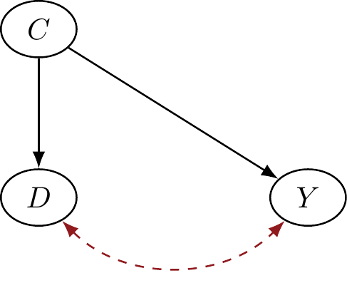
A directed acyclic graph draws our causal assumptions — and makes the source of the bias visible.

Reading a DAG

• Nodes = variables; arrows = causal effects.
• A backdoor path links \(D\) and \(Y\) starting with an arrow into \(D\) (Pearl, Glymour, and Jewell, 2016; Breen, 2022).
• A confounder \(C\) sits on a backdoor path — it makes \(D\) and \(Y\) correlate without any causal arrow between them. Confounder bias is selection bias.

The red dashed arrow is not really part of the DAG — it just marks the spurious \(D\)–\(Y\) correlation that the backdoor path through \(C\) produces.

A DAG maps your causal assumptions, not your data. The puppet metaphor works well: grab a node, shake it, and the movement travels along the arrows. Shake \(C\) and both \(D\) and \(Y\) move together — that is the spurious correlation. Shake \(D\) and \(Y\) does not move at all, because there is no arrow between them. A confounder is just a variable sitting on such a backdoor path.

Our case: a confounded correlation

Plausibly, German citizenship shapes both whether people follow German news and how much discrimination they encounter.

It opens a backdoor path — so the raw news–discrimination correlation is (at least partly) spurious, exactly the selection bias the balance table revealed.

Now make it concrete with our own case. German citizenship plausibly drives both whether people follow German news and how much discrimination they actually encounter. Trace the backdoor path with your finger: reads news ← German citizen → discrimination. That path on its own could produce the negative correlation we saw — no causal arrow required. And this is exactly the imbalance the balance table found.

The verdict: correlation ≠ causation

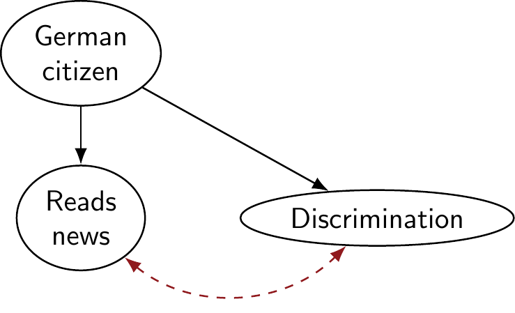
Correlation ≠ causation. The baseline \(Y_0\) differs between the groups we compare, because confounders sort people into and out of reading the news.

Ice-cream sales and shark attacks correlate — but temperature drives both. A raw correlation is a starting point, never a conclusion. The rest of this course is about earning the causal reading.

Close the loop: they now know why this flat line cannot be read causally — confounders sort people into and out of reading the news, so the baselines differ. Ice cream and shark attacks is the throwaway example if anyone still resists. Then bridge to next week: if the problem is that the groups differ to begin with, the fix is to make them comparable — which is what randomisation does.

Your turn: exercise 2

You draw the DAG and run a balance test yourself — is racial appearance balanced across news readers?

Open exercise 2 in a new tab ↗

Today’s general lessons

1. A causal claim is a counterfactual claim — it compares an outcome with a treatment to the same outcome without it.

2. Potential outcomes (\(Y_0\), \(Y_1\)) make this precise; a personal causal effect is \(Y_1 - Y_0\). The fundamental problem: one of them is always missing.

3. The average causal effect is the average of those personal effects.

4. A naïve comparison of groups usually is not the causal effect — it adds selection bias: the groups differ in their baseline \(Y_0\).

5. A balance test exposes observed imbalance; a DAG shows why — a confounder on a backdoor path. Confounder bias is selection bias.

Run through this fast — they are tired by now. If only one sentence survives the day, make it this one: an observed difference in means is a causal effect plus selection bias, and everything we do from here on is about forcing that second term to zero.

Check yourself: today’s goals

• Write a causal hypothesis as a difference of two potential-outcome averages — and say which term is never observed.
• Explain, using Ferda & Tuki, how an observed group difference splits into a causal effect plus selection bias.
• Draw the news → discrimination DAG with a confounder, and say what a balance test would show.

Shaky on any of these? That is what this week’s Absalon quiz and the Friday exercise class are for.

Today’s important functions

• rowMeans(select(., ...)): average several items into one index (same units).
• estimatr::lm_robust(y ~ d, weights = ...): weighted OLS with robust standard errors.
• modelsummary::datasummary_balance(~ group, data = ...): a balance table across two groups (rename your weight column to weights).

References

Breen, R. (2022). “Causal inference with observational data”. In: Handbook of Sociological Science: Contributions to Rigorous Sociology. Ed. by K. Gërxhani, N. de Graaf and W. Raub. Edward Elgar Publishing, pp. 272-286.

Pearl, J., M. Glymour, and N. P. Jewell (2016). Causal Inference in Statistics - A Primer. 1.th ed. Chichester, West Sussex: Wiley.

Schaeffer, M. and J. Kas (2024). “The integration paradox: Does awareness of the extent of ethno-racial discrimination increase reports of discrimination?” In: Political Psychology.

Schaeffer, M., J. Kas, and P. Hagedorn (2023). “The Association between Actual and Perceived Discrimination (APAD): Technical Report”. In: SocArXiv.