Randomness & Statistical Inference

What a random sample can — and cannot — tell us

Merlin Schaeffer · Department of Sociology

2026-07-23

By the end of today you can …

1. explain why we rely on random samples — and how weights repair imperfect randomness;

2. see that every sample carries sampling error, and estimate it with a standard error;

3. use confidence intervals and hypothesis tests to say what a sample can — and cannot — generalise.

One part of today’s lecture per goal. Our running question: do better-educated people generally believe more in the political system’s responsiveness?

Random samples & weights

Part 1 of 3

All our data are samples. To generalise from them safely, we lean on one idea: randomness.

The research question of the day

Do better-educated people generally believe more strongly that the political system is responsive — that people like them have a say?

Political efficacy: the belief that one’s voice counts in politics.

Discuss: we only ever have data on some people, in some year. What has to be true about those people for us to trust a general answer?

Note the word “generally” in the question — that single word is what makes today necessary. We have 1,500-odd Danes from one year, and we want to say something about people in general. Let them answer the blue box; whatever they say will be some version of “the sample has to be like everyone else”, which is precisely Part 1.

Preparation

• Packages for today’s session
• Get the ESS data

pacman::p_load(
  tidyverse,    # Data manipulation and visualization
  haven,        # Read SPSS/Stata files & handle labelled data
  estimatr,     # OLS with robust standard errors (for weights)
  modelsummary  # Nicely formatted regression tables
)

Download ESS9e03_1.sav from Absalon into your course project folder, then:

ESS <- read_spss("ESS9e03_1.sav") %>%
  filter(cntry == "DK") %>% # Keep only the Danish respondents
  # A minimal set of variables for today
  select(idno, pspwght, gndr, eduyrs, agea,
         psppsgva, trstlgl, trstplc) %>%
  mutate(across(c(psppsgva, trstlgl, trstplc, pspwght),
                zap_labels),                # Labelled -> numeric
         eduyrs = pmin(pmax(eduyrs, 9), 21), # Censor at 9 & 21 years
         gndr   = as_factor(gndr)) %>%
  drop_na() # Drop cases with missing values

Why do we study samples at all?

(1) Populations are too large to survey everyone.

(2) Even with data on everyone, we care about general patterns and social mechanisms — not just this year’s Danes or today’s countries.

So we treat any data set — even a full register — as one sample drawn from an unobservable “super-population”.

Reason two is the surprising one, so spend the time there. Even with Danish register data on everybody, we would still be doing inference — because we care about the social mechanism, not about these particular Danes in this particular year. That is why the super-population idea matters and why “but I have the whole population” is not an escape from statistics.

Source: Wikipedia

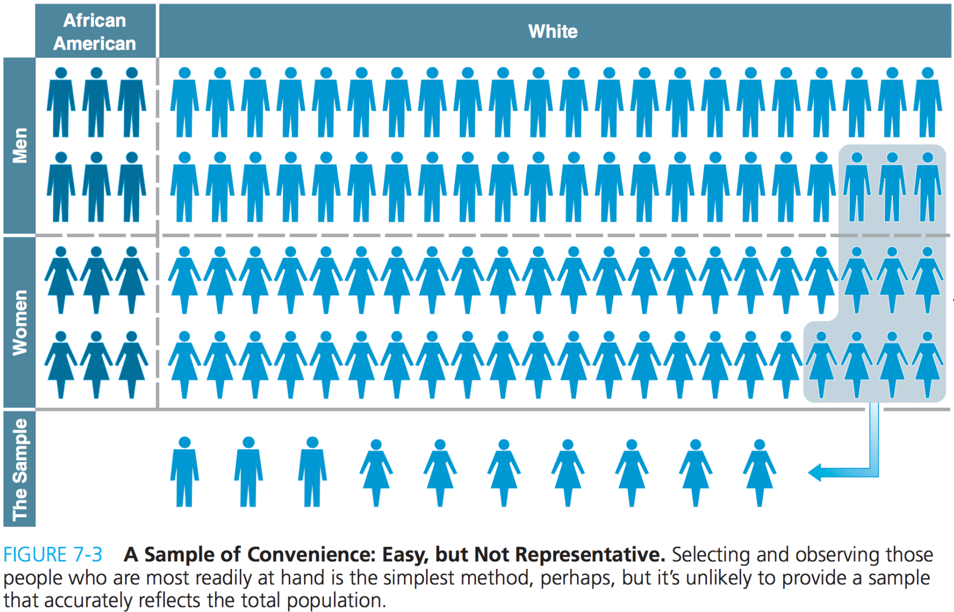
Convenience samples mislead

A good sample is representative — it mirrors the super-population.

Discuss: you snowball-sample starting from your best friend. What bias creeps in — and who gets left out?

Your friends resemble you (age, education, city, politics). Whole groups are systematically missing — the sample is biased before you compute anything.

Make it personal — ask them who their snowball sample would actually reach, and who it would never touch. The key phrase for the reveal: the sample is biased before you compute anything. No amount of clever analysis repairs a sample that never contained the people you care about.

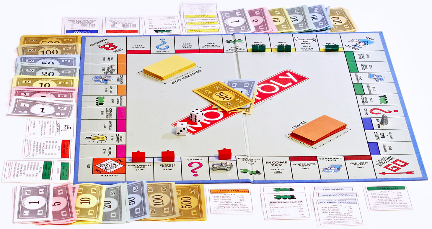
Randomness = fairness

Why do so many games use dice, coins, shuffled cards?

Fairness: a random draw gives everyone the same chance, regardless of who they are. No player — and no social group — can be systematically forgotten.

A random sample is the equivalent of stirring the soup before you taste it: one spoonful then represents the whole pot.

The soup metaphor is the one they will remember, so say it twice: stir the pot, and one spoonful tells you about the whole thing — and note that the size of the spoon matters far less than the stirring. Same logic as the coin in a fair game: randomness is not about being unpredictable, it is about being fair to every group.

But participation is not random

Who answers a survey is never a perfect coin flip — some groups are harder to reach, or more willing to respond.

We repair this after the fact with post-stratification weights.

What is a weight?

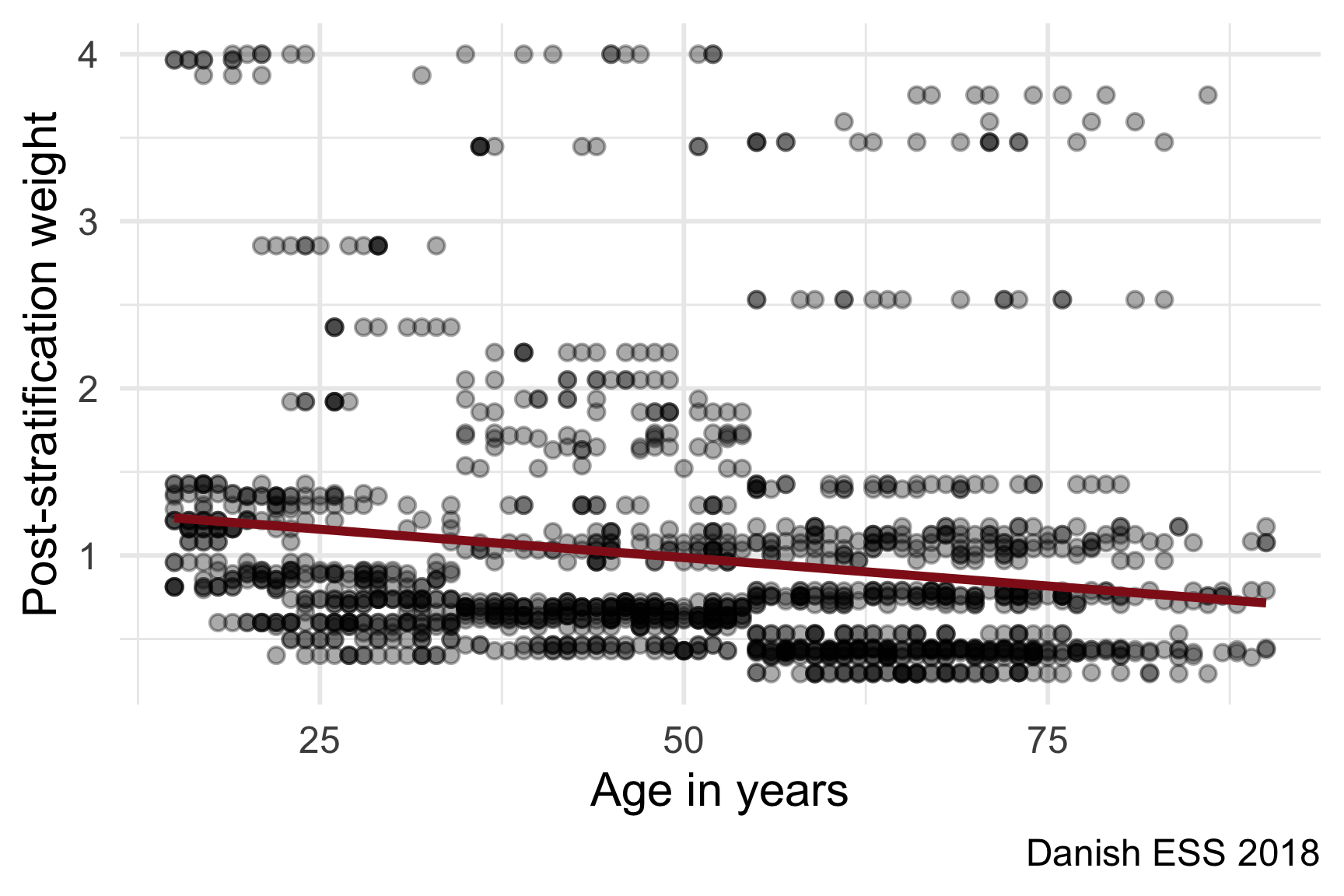
A weight reflects how much a case should count, to undo over- or under-sampling.

In a perfect random sample every case has weight 1. If older people are over-represented, we give them a weight below 1; under-represented groups get a weight above 1.

Discuss: the plot shows the ESS weights by age. Why might survey researchers down-weight older respondents here?

Define it in one line: a weight is how many people in the population this respondent stands for. Then the blue box — older people are easier to reach and more willing to answer, so they are over-represented and get weighted down. Ask what would happen to our education result if the over-represented group also differed in education; that is the whole reason weights exist.

How weights work: a worked example

Imagine a patriarchal ballot on women’s driving rights, where a man’s vote counts double a woman’s.

Gender	Vote	Voted yes	Weight
man	No	0	2
man	Yes	1	2
woman	Yes	1	1
woman	Yes	1	1
woman	No	0	1

Discuss: ignoring weights, what share voted “Yes”?

Three equivalent ways to get the weighted share of “Yes”:

• By hand
• With vectors
• Built-in

# (yes × weight) summed, over total weight
((1*2 + 1 + 1) / (2 + 2 + 1 + 1 + 1)) * 100
# [1] 57.1

yes    <- c(0, 1, 1, 1, 0)
weight <- c(2, 2, 1, 1, 1)
sum(yes * weight) / sum(weight) * 100
# [1] 57.1

weighted.mean(x = yes, w = weight) * 100
# [1] 57.1

Get the unweighted answer out of them first — 60% voted yes — then run the weighted version and watch it drop. The deliberately unpleasant framing (a man’s vote counting double) makes the mechanics obvious: weighting is just counting some rows more than others. Three routes to the same number, so nobody has to take weighted.mean() on faith.

Weights can be powerful

With the right weights, even a wildly non-representative sample can forecast well.

Wang, Rothschild, Goel, and Gelman (2015) predicted the 2012 US election from Xbox gamers — young, male, unrepresentative — reweighted to the electorate.

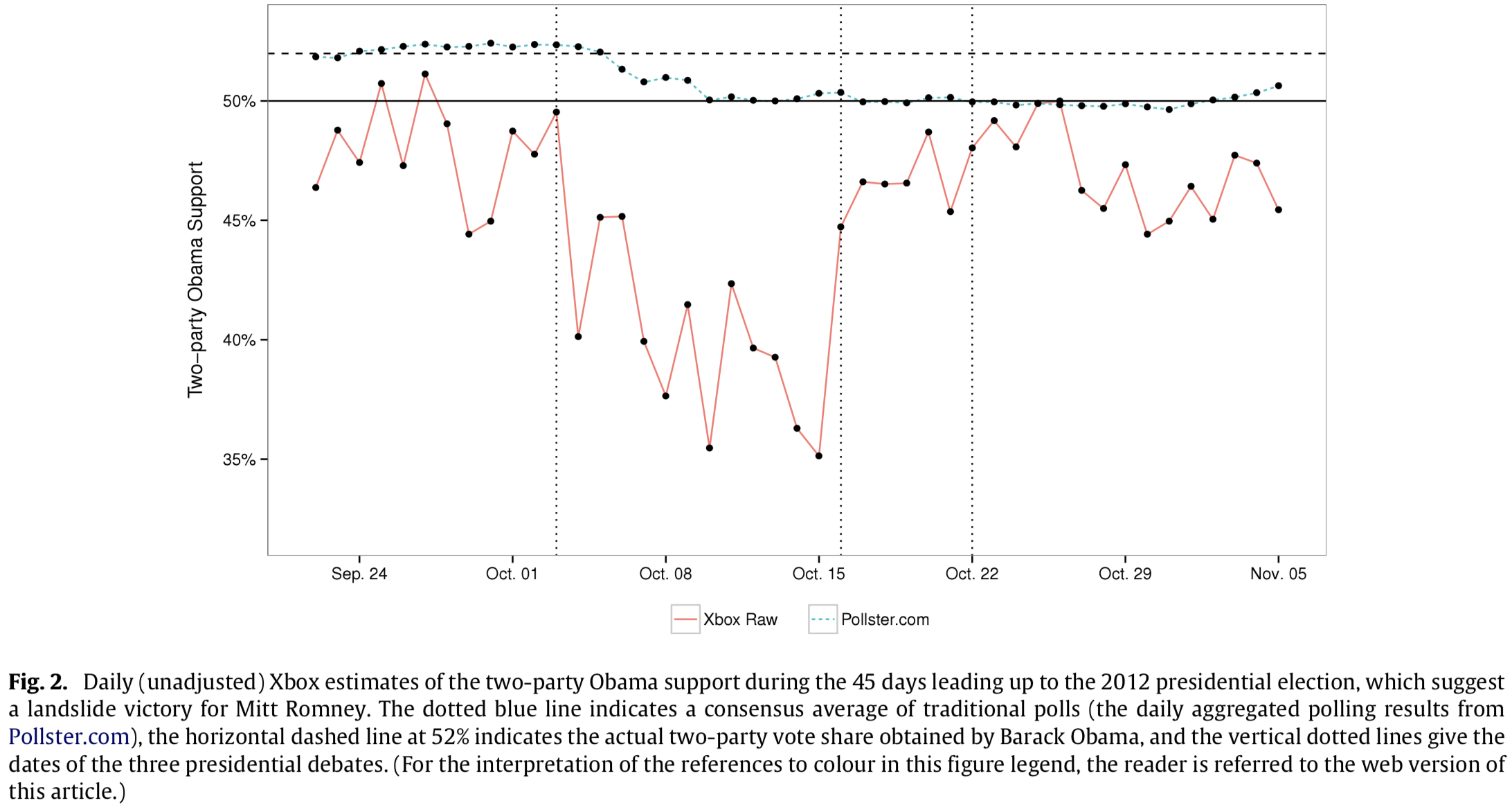
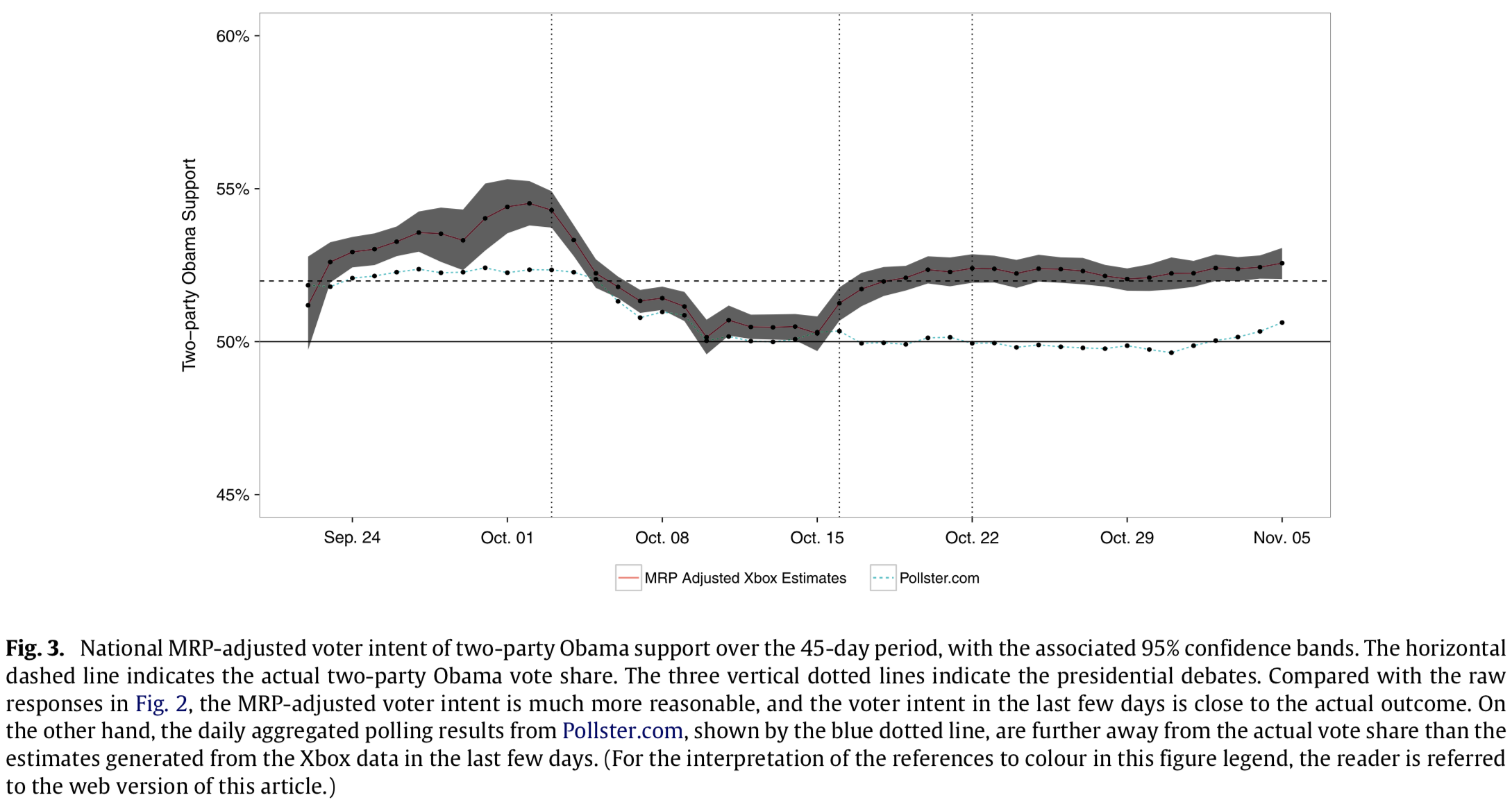
Source: Wang, Rothschild, Goel et al. (2015)

A genuinely fun result — Xbox gamers are about as unrepresentative of the US electorate as a sample can get, young and overwhelmingly male, and reweighted they still called the 2012 election well. Use it to make the honest point and its limit: weights repair imbalance on characteristics you can measure and know the population totals for. They cannot conjure back people the sample never reached at all.

Using weights in regression

Most R functions take a weights argument. For weighted OLS use estimatr::lm_robust().

Weights make the residuals heteroscedastic — which breaks a standard OLS assumption. lm_robust() fixes the standard errors for us.

• Table
• R code

	Unweighted	Weighted
(Intercept)	2.199	2.378
eduyrs	0.039	0.025
Num.Obs.	1511	1511
R2	0.026	0.010

mod_unw <- lm_robust(psppsgva ~ eduyrs, data = ESS)
mod_wt  <- lm_robust(psppsgva ~ eduyrs, data = ESS, weights = pspwght)

modelsummary(
  list("Unweighted" = mod_unw, "Weighted" = mod_wt),
  statistic = NULL,
  gof_map = c("nobs", "r.squared"),
  output = "kableExtra"
)

Practical takeaway: add weights = and switch to lm_robust(). Explain why the switch is needed — weighting makes the residuals heteroscedastic, which breaks a standard OLS assumption, and lm_robust() repairs the standard errors. Compare the two columns: the coefficients move a little, which is exactly the correction doing its job.

Sampling error & the standard error

Part 2 of 3

Randomness removes bias — but a random sample is still noisy. How noisy, exactly?

A thought experiment: pretend we see everyone

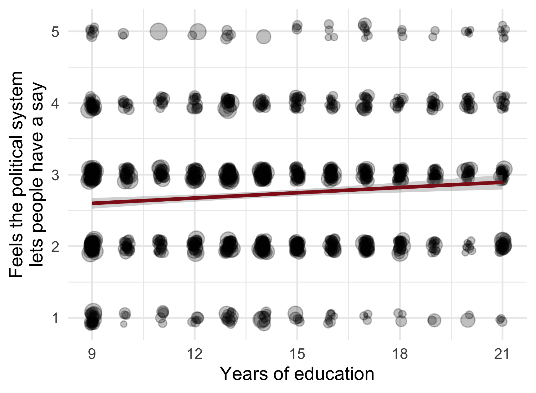
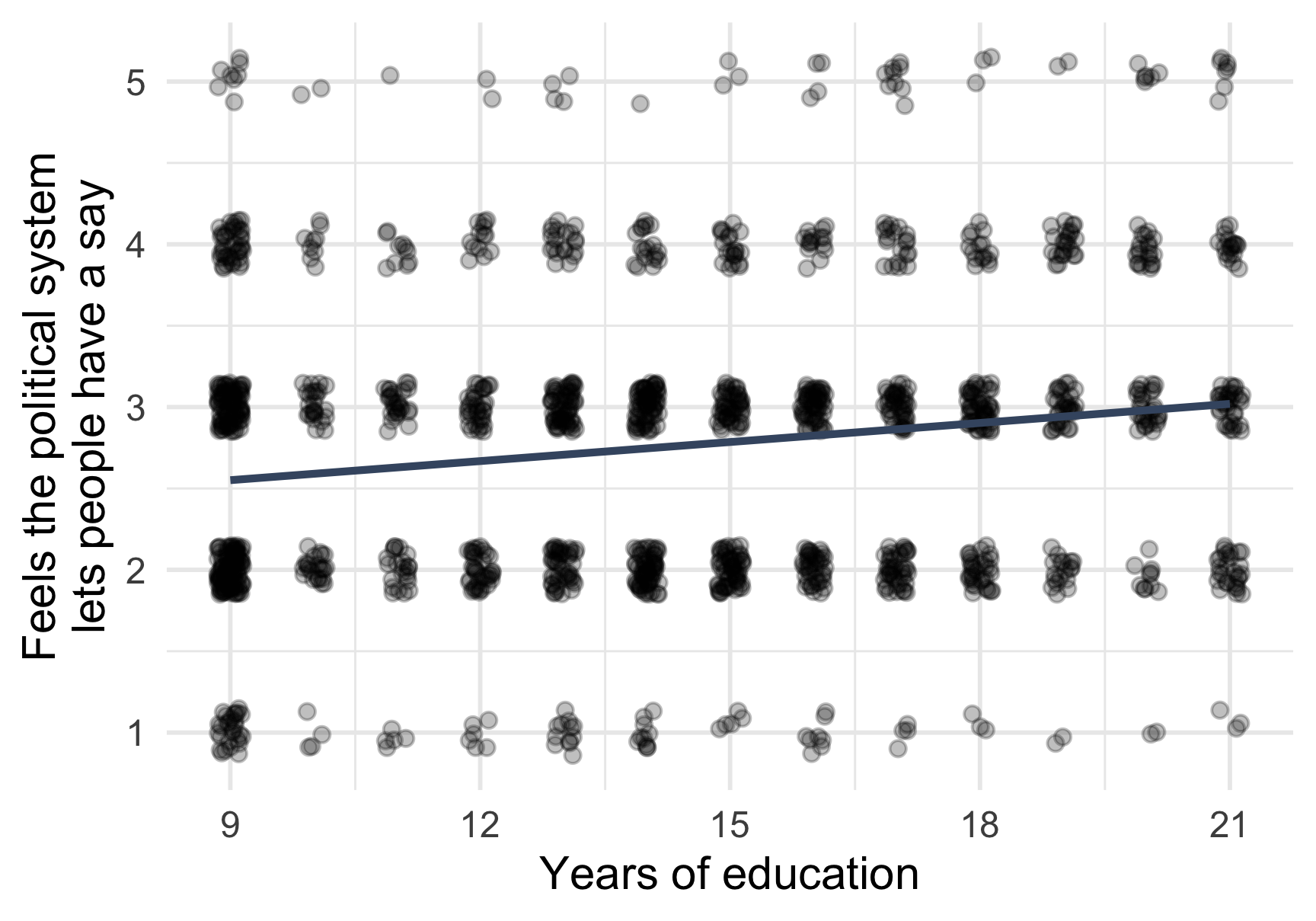
Suppose the Danish ESS (1511 people) were our whole super-population.

Then we could calculate the true slope of political efficacy on education (blue line): \[\beta = 0.039\]

No weights here — this is a make-believe population.

Set the fiction up carefully, because the next six slides depend on it: pretend these 1,500 Danes are the entire world. Under that pretence we can compute the true β — the blue line — which we never actually get in real research. Keep pointing back at the blue line; it is the fixed truth everything else will scatter around.

Now draw one small sample

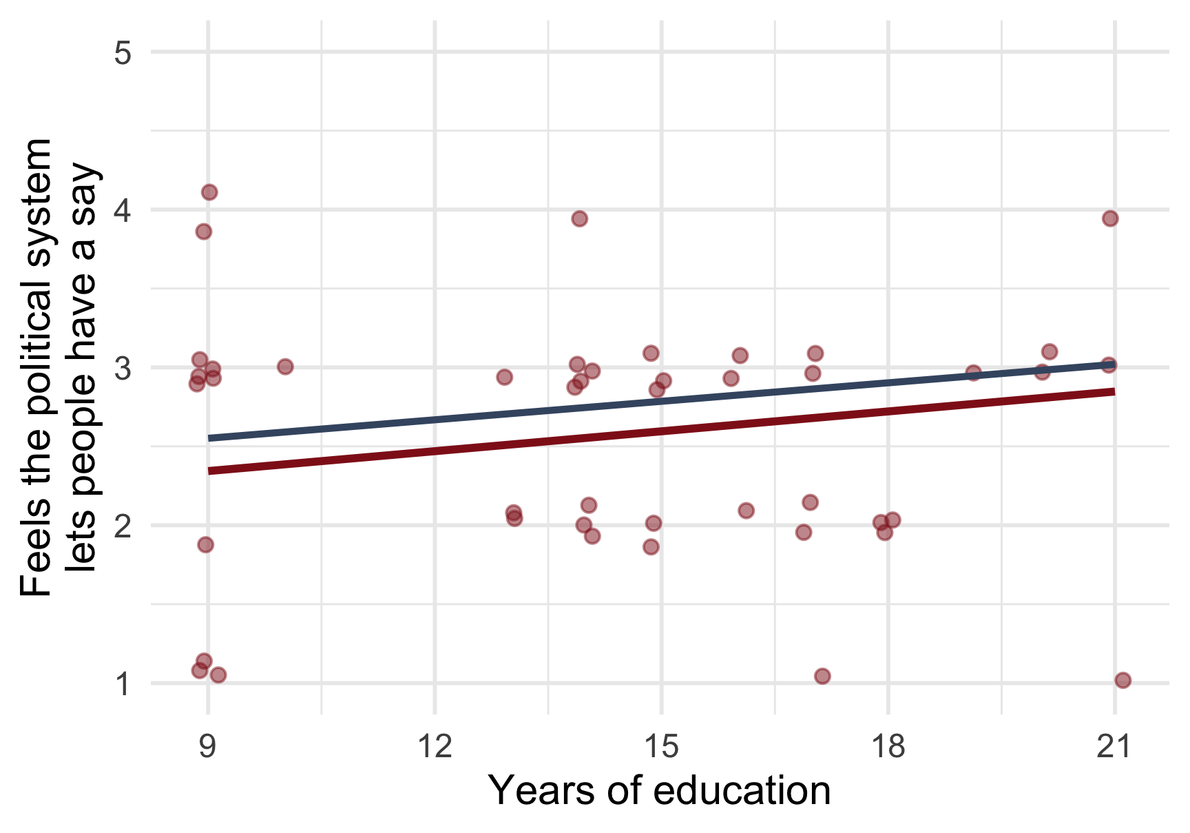
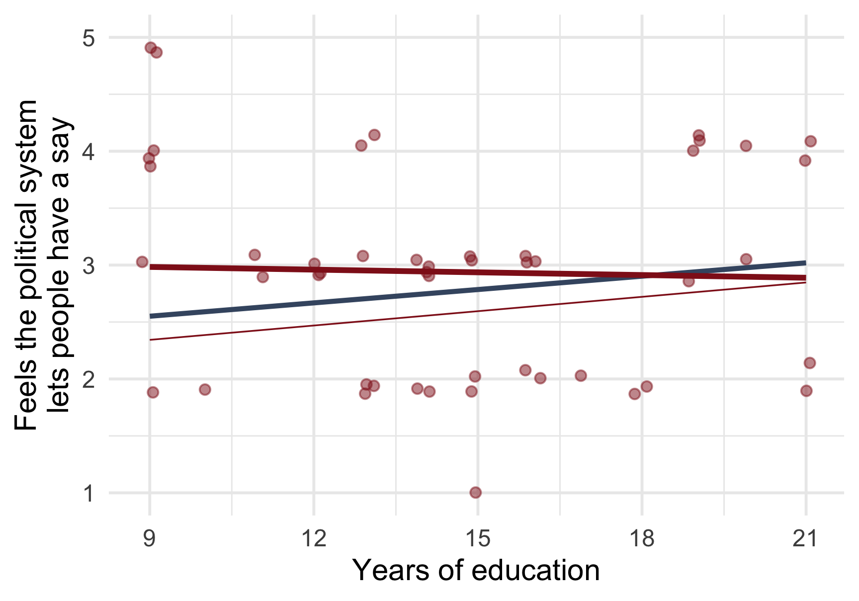
We rarely see the population — usually just a sample. Take 50 people at random:

set.seed(1261990)
ESS_sample <- ESS %>% sample_n(50)

The sample’s own regression line (red) gives \(\hat\beta = 0.042\) — not the true 0.039.

Another sample, another answer

Draw a different 50 people and the line moves again: \(\hat\beta = -0.008\).

Beware: each sample gives a different estimate. This scatter of estimates around the truth is sampling error — not a mistake, but the price of not seeing everyone.

Nothing was done wrong, and that is the lesson — same population, same code, different 50 people, different answer. Insist on the vocabulary: this is sampling error, not a mistake. It is the unavoidable price of not seeing everyone, and the rest of the lecture is about measuring it rather than eliminating it.

… and again, and again

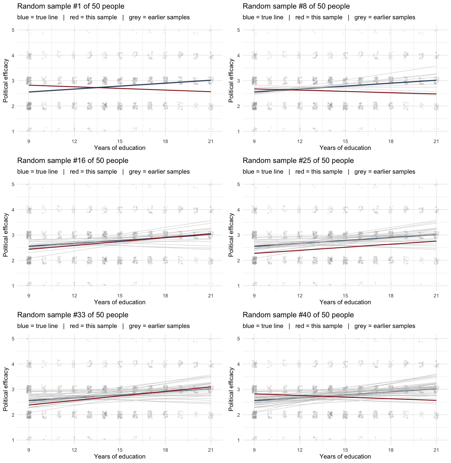
Keep drawing fresh samples of 50. Every red line is a new random sample; the blue line is the unchanging truth.

The lines fan out around the true line. That fan is the sampling error — visible, and (as we’ll see) predictable.

Let the animation run twice and just narrate it — every red line is one researcher’s honest study. Two things to point out: they fan out around the blue truth rather than drifting off it, and the fan has a definite width. Both matter: unbiased, but noisy, and the noise is regular enough to be measured.

Do it 1000 times: the sampling distribution

• The idea
• Watch it build
• Histogram
• It’s Normal!
• Small samples: the t

Repeat “draw 50, estimate \(\hat\beta\)” 1000 times and collect all the estimates. Their spread is the sampling error — and it has a beautiful, predictable shape.

set.seed(1261990)
sample_betas <- replicate(1000, {          # 1000 repetitions of …
  s <- ESS %>% sample_n(50)                # … draw 50 people
  coef(lm(psppsgva ~ eduyrs, data = s))["eduyrs"] # … store the slope
})
sd(sample_betas) # The true sampling error
# [1] 0.0367

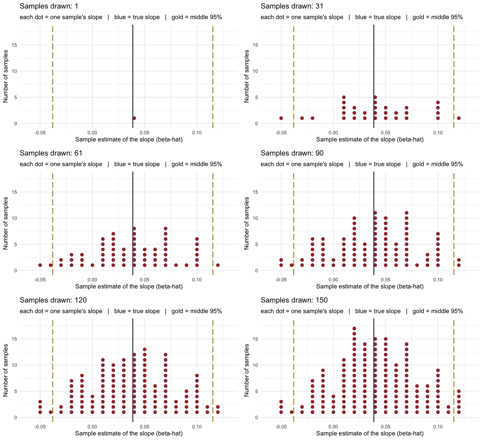
Each dot is one sample’s slope. As they pile up, a bell curve emerges around the true \(\beta\).

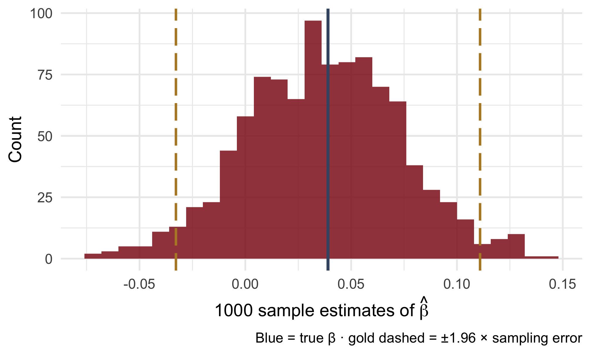
The estimates pile up in a Normal (bell) curve around the truth. We know its areas exactly:

• \(\pm 1.65 \times\) SD covers the middle 90%
• \(\pm 1.96 \times\) SD covers the middle 95%

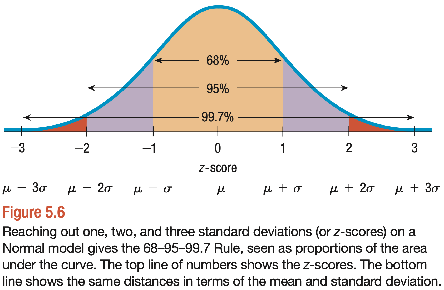
Source: Veaux, Velleman, and Bock (2021)

With small \(n\), the curve has slightly fatter tails — the \(t\)-distribution. Its critical value depends on the degrees of freedom (\(n\) − parameters):

# 95% critical value, df = 50 − 2
qt(p = 0.975, df = 48)
# [1] 2.01

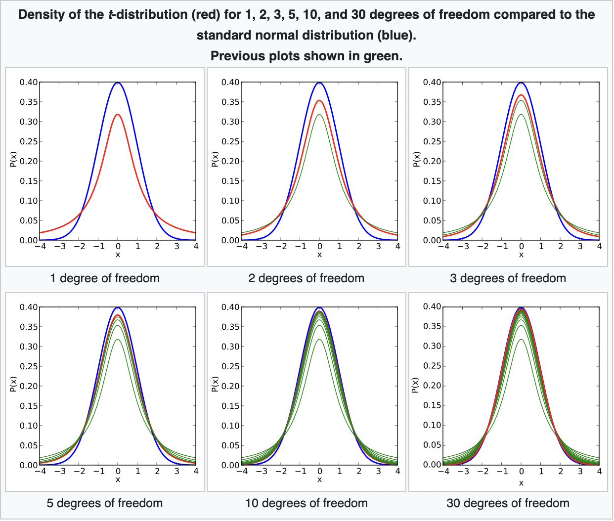
Source: Wikipedia

The crux of the lecture — go slowly and use the “watch it build” tab. Each dot is one whole study; say that out loud, because students routinely think a dot is a person. As the dots pile up a bell curve appears around the truth, and once we know it is Normal we know its areas exactly: ±1.96 SD covers the middle 95%. The \(t\) tab is a footnote — same idea, slightly fatter tails when \(n\) is small.

The catch — and Gauss’s gift

Discuss: in real research we get one sample. We can’t draw 1000. So how could we possibly know the sampling error?

Thanks to Carl Friedrich Gauss, we can estimate the sampling error from a single sample. That estimate is the standard error \(\hat\sigma\).

For an OLS slope: \[\hat{\sigma}(\hat\beta) = \sqrt{\frac{1}{n-2}\,\frac{\text{SD}(e)}{\text{SD}(x)}}\]

	 50-person sample
(Intercept)	1.965
	(0.530)
eduyrs	0.042
	(0.036)
Num.Obs.	50
R2	0.027

The estimated SE from this one sample (0.036) is remarkably close to the true sampling error from 1000 samples (0.037).

Ask the blue-box question and let it land as a real problem: everything so far needed 1000 samples, and in real research we get one. Then the payoff — Gauss showed the spread of that 1000-sample distribution can be estimated from a single sample. Put the two numbers side by side and let them see how close they are. That is what a standard error is, and it is why the SE column in every table they have ever seen is not magic.

Your turn: samples & weights

Open exercise 1 in a new tab ↗

Break

Confidence intervals & hypothesis tests

Part 3 of 3

The standard error turns a single estimate into an honest statement of uncertainty.

95% confidence intervals

Combine the estimate with its standard error:

\[\hat\beta \pm \text{critical value} \times \hat\sigma\]

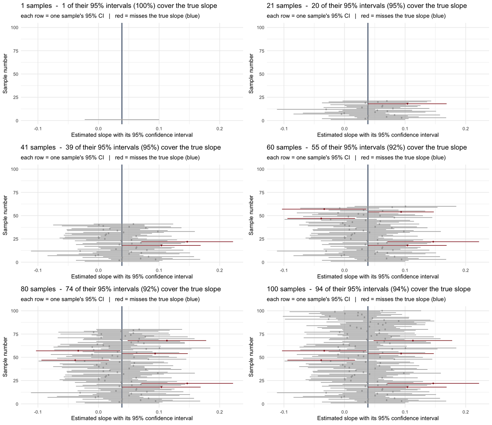
What “95%” means: if we drew samples over and over and built this interval each time, 95% of those intervals would contain the true \(\beta\) — the blue line. It is a statement about the procedure, not any single interval.

Watch the intervals accumulate: only about 1 in 20 (the red ones) misses the truth.

Be pedantic here, because the wrong version is everywhere: 95% is a property of the procedure, not of the one interval in front of you. Run the animation and count the red misses — about 1 in 20, exactly as advertised. The sentence to forbid: “there is a 95% chance the true value is in this interval.” The true β is fixed; it is our intervals that jump around.

Confidence intervals, hands-on

Play with samples, coverage, and interval width yourself:

Uncertainty, drawn

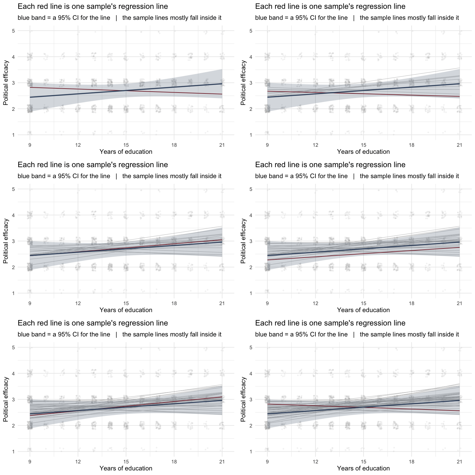
geom_smooth(method = "lm") shades the 95% CI around the line — wide where data are thin, narrow where they are dense.

ggplot(ESS_sample, aes(y = psppsgva, x = eduyrs)) +
  geom_jitter(alpha = 1/3,
              width = 0.1, height = 0.1) +
  geom_smooth(method = "lm", color = "#901A1E") + # 95% CI band
  ylim(1, 5) +
  labs(y = "Political efficacy",
       x = "Years of education")

The band is exactly the region where those sampled regression lines plausibly lie — watch them fall inside it.

This connects the grey band they have been drawing since Lecture 2 to everything we did today. The animation is the point: the accumulating sample lines are the same red lines from earlier, and the band is where they live. Also note the shape — wide where the data are thin, narrow where they are dense, which is just sampling error depending on how much information sits at each x.

Hypothesis tests: argue with an opponent

The debate of Socrates and Aspasia

Research is a debate with a sceptic who dismisses your finding:

“Sure, your educated respondents scored higher — but that’s just a fluke of your sample. Really there’s no difference at all.”

\[\underbrace{H_{0}}_{\text{the } H_{\text{opponent}}}:\ \beta_{\text{education}} = 0\]

We test whether the data can overturn this null.

Frame testing as an argument rather than a ritual: there is a sceptic in the room who says your finding is just a fluke of your sample. \(H_0\) is their position, not yours. Everything that follows is the machinery for deciding whether the data embarrass them. Students who see the null as an opponent stop mixing up which hypothesis is being tested.

The (weird) logic of a test

• \(H_0\): the sun is shining.

• I see 5 kids walking to school with umbrellas. How likely is that if the sun is really shining?

• If that probability is below 5%, I stop believing \(H_0\) — I bet it’s raining.

Discuss: can you phrase your own everyday \(H_0\)-and-evidence example?

We never prove our hypothesis. We show the sceptic’s \(H_0\) makes the data too surprising to keep believing.

The umbrella example is worth acting out. Notice the direction of reasoning — we never prove it is raining; we show that the umbrellas would be too surprising if the sun were shining. Say the last line twice, because it is the sentence they get wrong in exams: a significant result is evidence against \(H_0\), never proof of \(H_1\).

Put it into practice

• \(t\) and \(p\)
• In one small sample
• The full sample

\(t\)-value \(= \dfrac{\hat\beta}{\hat\sigma}\) — how many standard errors the estimate sits from 0.

\(p\)-value — if \(H_0\) were true, the probability of an estimate this far from 0 (or further).

A small \(p\) (by convention \(< 0.05\)) means the data are hard to reconcile with \(H_0\) — evidence against it, not proof of \(H_1\).

ols <- lm_robust(psppsgva ~ eduyrs,
                 data = ESS_sample)
tidy(ols) %>%                    # Tidy result table
  filter(term == "eduyrs") %>%
  select(estimate, std.error,
         statistic, p.value)
#   estimate std.error statistic p.value
# 1    0.042     0.043     0.976   0.334

In our 50-person sample the estimate is positive but not significant — with so few people, sampling error is simply too large to rule out \(H_0\).

	Political efficacy
(Intercept)	2.378***
	(0.114)
eduyrs	0.025**
	(0.008)
Num.Obs.	1511
R2	0.010
+ p < 0.1, * p < 0.05, ** p < 0.01, *** p < 0.001

The \(t\)-value is just “how many standard errors from zero” — no more mysterious than that. The three tabs make the real point: the same effect is not significant in the 50-person sample and clearly significant in the full one. Nothing about the world changed, only how much sampling error we were carrying. Non-significant does not mean “no effect”; it can simply mean “not enough people”.

Learning goal achieved

Using the whole weighted sample, education predicts political efficacy:

• \(\hat\beta = 0.025\) per year of education,
• standard error \(0.008\),
• \(t = 3.2\), \(p = 0.0015\).

Answer: yes — better-educated Danes believe significantly more in the political system’s responsiveness. The effect is small per year, but clearly not zero.

Close the loop on the opening question and make them read all four numbers — estimate, SE, \(t\), \(p\) — as one sentence. Then add the honest caveats, since both matter: the effect is small per year of education, and significant is not the same as large. And it is not causal — education is not randomly assigned, which is where the next lectures go.

Your turn: inference

Open exercise 2 in a new tab ↗

Check yourself: today’s goals

Look back at the goals from the start of the lecture. Can you tick all three?

• Explain to your neighbour why a random sample beats a convenience sample — and what a weight repairs.
• Say, in one sentence, what a standard error estimates — using the word sampling distribution.
• Read a regression’s \(t\)- and \(p\)-value and state what they do (and don’t) let you conclude about \(H_0\).

Anything feel shaky? That is what this week’s Absalon quiz and the Friday exercise class are for.

Today’s important functions

1. haven::read_spss() + zap_labels(): read SPSS data and turn labelled columns numeric.
2. dplyr::sample_n(): draw a random sample of rows.
3. weighted.mean(), and the weights = argument: analyses that respect survey weights.
4. estimatr::lm_robust(..., weights =): weighted OLS with correct standard errors.
5. qt(): critical values from the \(t\)-distribution.
6. geom_smooth(method = "lm"): an OLS line with its 95% confidence band.
7. broom::tidy(): pull estimates, standard errors, \(t\)- and \(p\)-values into a tibble.

References

Veaux, D., Velleman, and Bock (2021). Stats: Data and Models, Global Edition. Pearson Higher Ed.

Wang, W., D. Rothschild, S. Goel, et al. (2015). “Forecasting elections with non-representative polls”. In: International Journal of Forecasting, pp. 980-991.