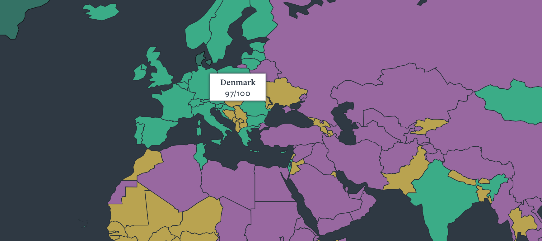
Correlation & OLS Regression

A recap — put to work on a real question

Merlin Schaeffer · Department of Sociology

2026-07-23

By the end of today you can …

1. download real data via APIs (World Bank, V-Dem) and join data sets in R;

2. describe a relationship with scatter plots, z-scores, and the correlation coefficient \(r\);

3. fit and interpret a bivariate OLS regression — and say when it may be read causally.

One part of today’s lecture per goal. Our running question: is there a liberty–equality trade-off?

The question & the data

Part 1 of 3

A real sociological debate — and the data to weigh in on it, four function calls away.

Remember? Citizenship rights across the world

Freedom House World Map

Last semester’s course mapped civic and political citizenship rights.

One may criticize: aren’t socialist countries better at providing social citizenship rights — affordable housing, healthcare, work, a minimum quality of life?

The research question of the day

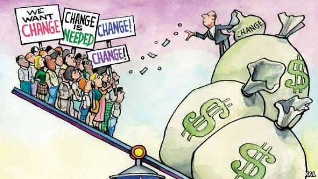
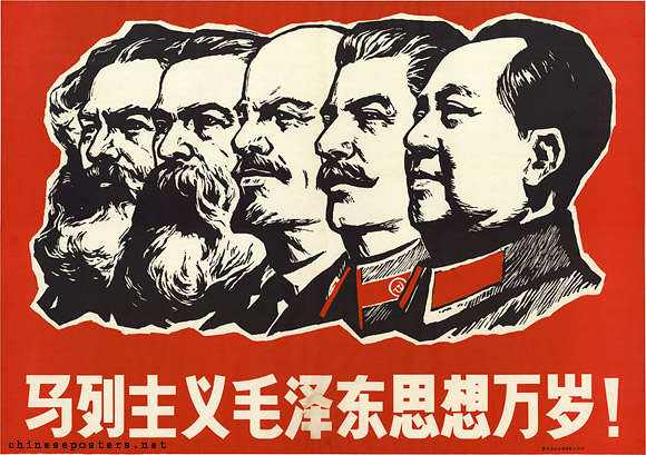
Research question of the day: is there a liberty–equality trade-off? Do state-owned (socialist) economies reduce poverty — at the price of fewer civil liberties?

An old and genuinely contested political claim: you can have equality or you can have liberty, but not both. Note that it is an empirical claim dressed as an ideological one — which means we can go and check it. Say up front that the answer today is descriptive, not causal; they will want to over-claim.

Our map for today: a triangle

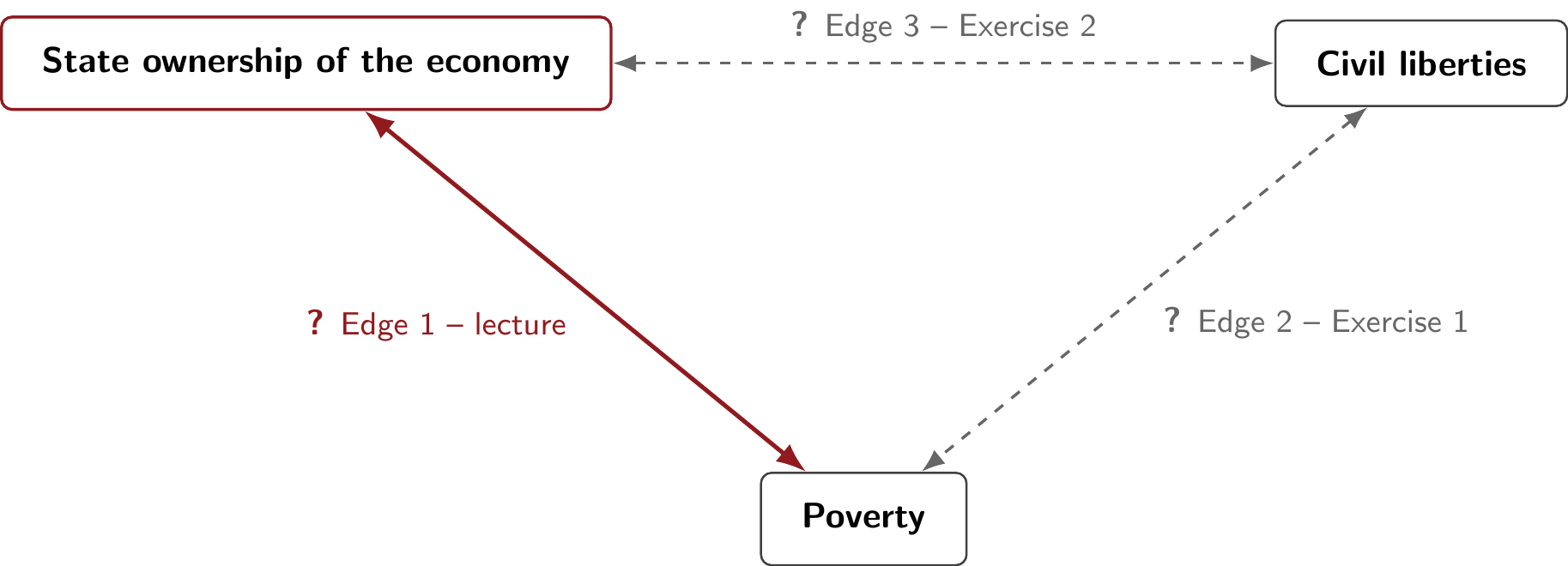
Three variables → three pairwise relationships. Only all three together answer the research question.

The thread for today: the lecture walks edge 1 step by step. You walk edges 2 and 3 in the exercises — with the same tools. The final slide assembles the verdict.

Spend a minute here — this triangle is the map for the whole day, exercises included. Three variables mean three pairwise relationships, and the research question needs all three. Tell them explicitly that the exercises are not busywork: without their two edges we cannot reach the verdict on the closing slide.

What is socialism — and how do we measure it?

Socialism (as an economic system): the means of production and distribution are
owned or controlled by the state or collectively — rather than privately.

\(\rightarrow\) The measurable core of the concept: state ownership of the economy.

We use the expert-coded V-Dem indicator state ownership of the economy (v2clstown) — available for virtually all countries since 1789 — and reverse it, so that higher = more state ownership.

Discuss: why not simply code countries that call themselves socialist — say, from Wikipedia’s list of socialist states?

Self-description is cheap talk — North Korea calls itself a Democratic People’s Republic. A good operationalisation is valid (measures what states do, not what they say), reliable (many independent country experts, aggregated by a measurement model), and comparable (one scale, all countries, all years).

This is the measurement slide, and it matters more than it looks. Ask the blue-box question and let someone defend the self-declared list before you reveal — the North Korea example usually ends the debate. Name the three criteria as the standard they should apply to any variable for the rest of the course: valid, reliable, comparable. Concepts are not variables until someone makes a defensible choice.

Preparation

• Packages for today’s session
• Working with APIs

pacman::p_load( # Load (and install if needed) several R packages
  tidyverse,    # Data manipulation and visualization
  wbstats,      # Download data from the World Bank API
  vdemdata,     # Varieties of Democracy (V-Dem) data
  estimatr,     # OLS with robust standard errors
  modelsummary, # Nicely formatted regression tables
  countrycode   # Easy recoding of country names
)

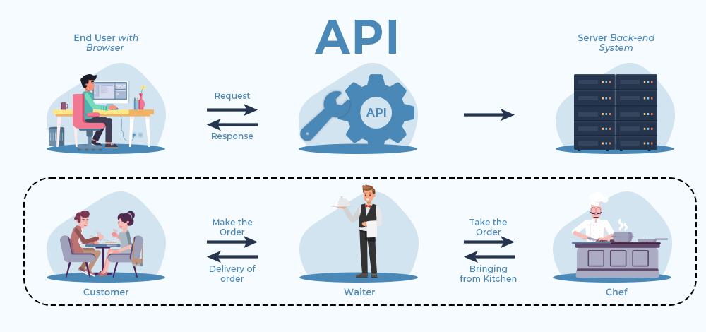
An API (Application Programming Interface) lets R talk directly to a data provider — no clicking, no downloading files by hand, fully reproducible.

(1) Varieties of Democracy data

Civil liberties — the V-Dem equality before the law and individual liberty index (v2xcl_rol): impartial administration, access to justice, property rights, freedom from torture and political killings, freedom of religion and of movement — for men and women. In T.H. Marshall’s terms, the civil dimension of citizenship rights.

State ownership of the economy: our reversed v2clstown (see previous slide).

• The data
• Get the data
• Sanity check
• … its R code

(Dat_vdem <- vdem %>% # The data ship with the vdemdata package
   as_tibble() %>%
   select(country = country_name, # Rename while selecting
          country_text_id, year,
          civ_liberties = v2xcl_rol,
          state_own_raw   = v2clstown) %>%
   # Reverse, so that higher = MORE state ownership
   mutate(state_ownership = -state_own_raw))
# # A tibble: 28,092 × 6
#    country country_text_id  year civ_liberties state_own_raw state_ownership
#    <chr>   <chr>           <dbl>         <dbl>         <dbl>           <dbl>
#  1 Mexico  MEX              1789           0.2          -0.2             0.2
#  2 Mexico  MEX              1790           0.2          -0.2             0.2
#  3 Mexico  MEX              1791           0.2          -0.2             0.2
#  4 Mexico  MEX              1792           0.2          -0.2             0.2
#  5 Mexico  MEX              1793           0.2          -0.2             0.2
#  6 Mexico  MEX              1794           0.2          -0.2             0.2
#  7 Mexico  MEX              1795           0.2          -0.2             0.2
#  8 Mexico  MEX              1796           0.2          -0.2             0.2
#  9 Mexico  MEX              1797           0.2          -0.2             0.2
# 10 Mexico  MEX              1798           0.2          -0.2             0.2
# # ℹ 28,082 more rows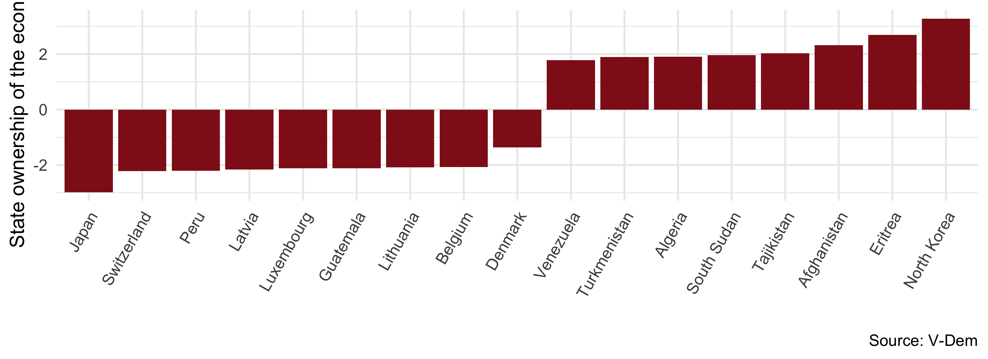

Reading the scale: it works like a z-score (today’s topic!): 0 ≈ the average country-year since 1789; around +2 ≈ heavily state-owned (North Korea); around −2 ≈ almost fully private (Switzerland).

Introduce the two V-Dem variables, then use the sanity-check tab as a habit rather than a slide: whenever you meet a new variable, look at its extremes and ask whether they make sense. North Korea at one end, Switzerland at the other, Denmark where you would expect — that is face validity, cheap and worth doing every time. It also previews the z-score, which is the next big idea.

Dat_vdem %>%
  filter(year == max(year)) %>%
  arrange(state_ownership) %>%
  # Keep the 8 lowest, the 8 highest, and Denmark
  filter(row_number() <= 8 | row_number() > n() - 8 |
           country == "Denmark") %>%
  ggplot(aes(y = state_ownership,
             x = reorder(country, state_ownership))) +
  geom_col(fill = "#901A1E") +
  labs(y = "State ownership of the economy", x = "",
       caption = "Source: V-Dem") +
  theme_minimal(base_size = 16) +
  theme(axis.text.x = element_text(angle = 60, hjust = 1))

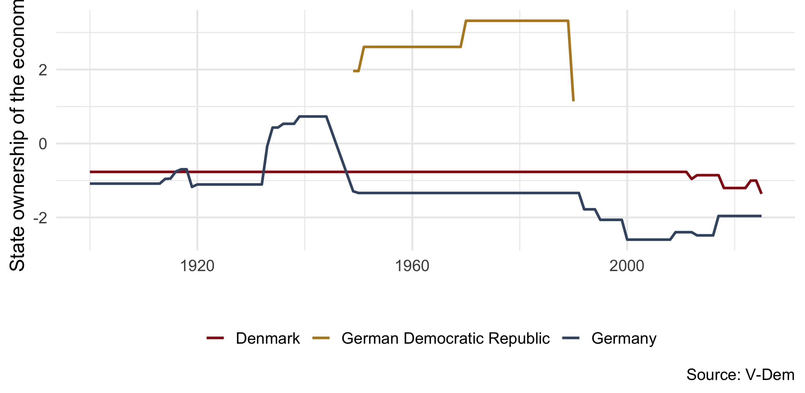
A case study: Denmark & the two Germanies

• State ownership since 1900
• … its R code
• Civil liberties since 1900
• … its R code
• What do we see?

ggplot(data = Dat_vdem %>%
         filter(country %in% c("Denmark", "Germany",
                               "German Democratic Republic"),
                year >= 1900),
       aes(y = state_ownership, x = year, color = country)) +
  geom_line(linewidth = 1) +
  scale_color_manual(values = c("Denmark" = "#901A1E",
                                "Germany" = "#425570",
                                "German Democratic Republic" = "#b5892c")) +
  labs(y = "State ownership of the economy", x = "", color = "",
       caption = "Source: V-Dem") +
  theme_minimal(base_size = 16) +
  theme(legend.position = "bottom")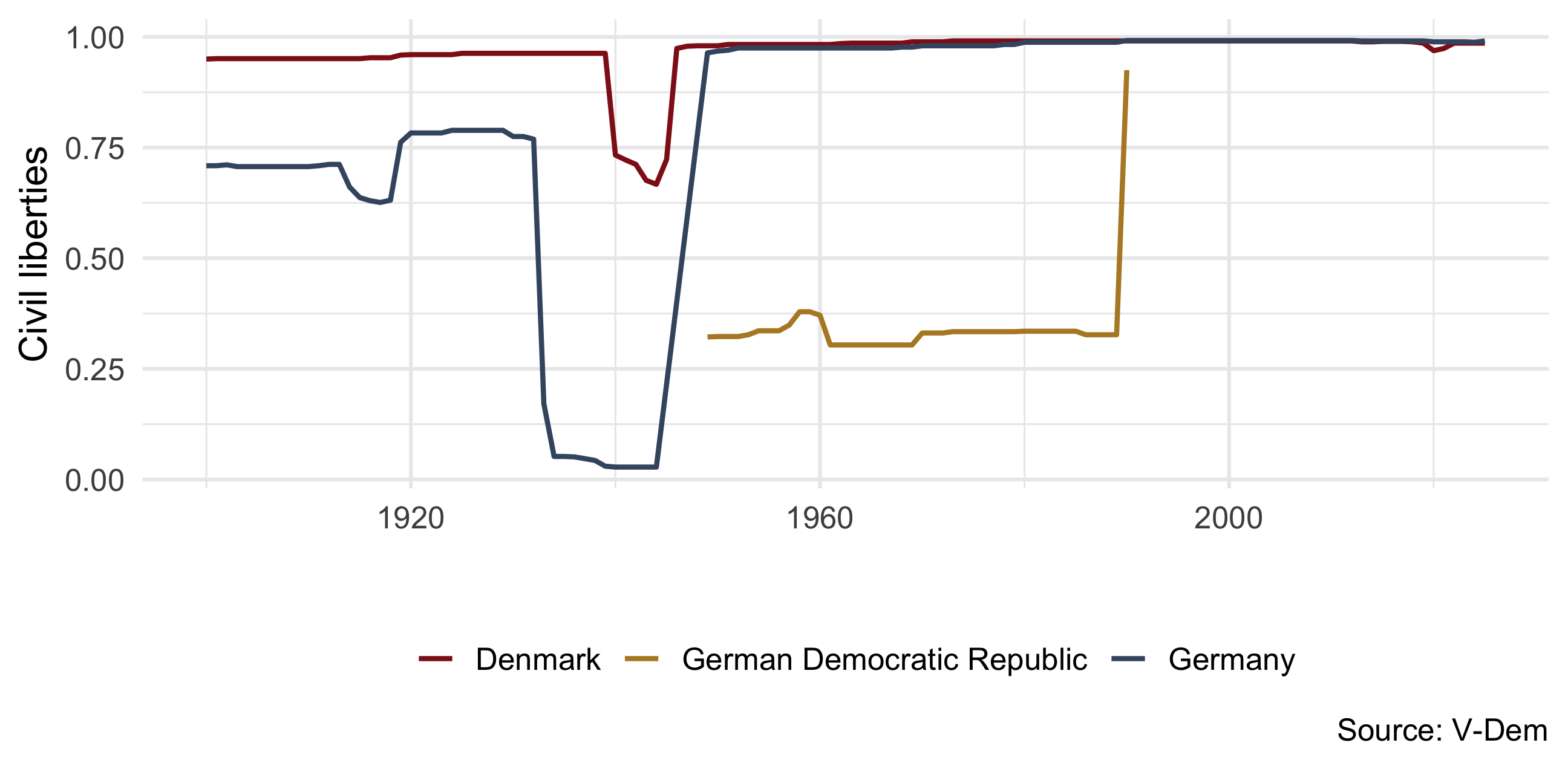

ggplot(data = Dat_vdem %>%
         filter(country %in% c("Denmark", "Germany",
                               "German Democratic Republic"),
                year >= 1900),
       aes(y = civ_liberties, x = year, color = country)) +
  geom_line(linewidth = 1) +
  scale_color_manual(values = c("Denmark" = "#901A1E",
                                "Germany" = "#425570",
                                "German Democratic Republic" = "#b5892c")) +
  labs(y = "Civil liberties",
       x = "", color = "", caption = "Source: V-Dem") +
  theme_minimal(base_size = 16) +
  theme(legend.position = "bottom")

Discuss: socialist East Germany (1949–1990) in both plots — what happens to state ownership and to civil liberties while the GDR exists, and after 1990? What does this one case suggest about our research question?

The GDR ran a far more state-owned economy and offered far fewer civil liberties than West Germany or Denmark — one historical case previewing edge 3 of our triangle. But one case is an anecdote; now we test the pattern across all countries.

A natural comparison: two Germanies, one nation, split for forty years. Let them read both series and describe what happens in 1949 and again after 1990. Then the methodological turn, which is the real point — this is a vivid anecdote, and one case cannot establish a pattern. That is exactly why we now go to all countries at once.

(2) World Bank data: poverty across the world

• Searching the WB archive
• Use the WB API
• What does “$3.00 a day” mean?
• Poverty across the world

With wb_search() you can search the World Bank archive for any keyword:

(wb_poverty_archive <- wb_search("Poverty")) # Search the WB data bank
# # A tibble: 702 × 3
#    indicator_id         indicator                               indicator_desc                                     
#    <chr>                <chr>                                   <chr>                                              
#  1 1.0.HCount.1.90usd   Poverty Headcount ($1.90 a day)         The poverty headcount index measures the proportio…
#  2 1.0.HCount.2.5usd    Poverty Headcount ($2.50 a day)         The poverty headcount index measures the proportio…
#  3 1.0.HCount.Mid10to50 Middle Class ($10-50 a day) Headcount   The poverty headcount index measures the proportio…
#  4 1.0.HCount.Ofcl      Official Moderate Poverty Rate-National The poverty headcount index measures the proportio…
#  5 1.0.HCount.Poor4uds  Poverty Headcount ($4 a day)            The poverty headcount index measures the proportio…
#  6 1.0.HCount.Vul4to10  Vulnerable ($4-10 a day) Headcount      The poverty headcount index measures the proportio…
#  7 1.0.PGap.1.90usd     Poverty Gap ($1.90 a day)               The poverty gap captures the mean aggregate income…
#  8 1.0.PGap.2.5usd      Poverty Gap ($2.50 a day)               The poverty gap captures the mean aggregate income…
#  9 1.0.PGap.Poor4uds    Poverty Gap ($4 a day)                  The poverty gap captures the mean aggregate income…
# 10 1.0.PSev.1.90usd     Poverty Severity ($1.90 a day)          The poverty severity index combines information on…
# # ℹ 692 more rows

# Download from the World Bank API; if it is unreachable, fall back to a
# cached copy so the analysis still runs (smart habit for any live data!)
poverty_raw <- tryCatch(
  wb_data("SI.POV.DDAY",                # Extreme poverty: below $3.00 a day (2021 PPP)
          start_date = 1972, end_date = 2025),
  error = function(e) readRDS("data/wb_poverty_raw.rds")
)

(Dat_poverty <- poverty_raw %>%
   rename(poverty = SI.POV.DDAY,
          year = date,
          country_text_id = iso3c) %>%
   select(country_text_id, year, country, poverty) %>%
   drop_na(poverty) %>%
   group_by(country) %>%
   filter(year == max(year)) %>% # Most recent estimate per country
   ungroup())
# # A tibble: 171 × 4
#    country_text_id  year country    poverty
#    <chr>           <dbl> <chr>        <dbl>
#  1 ALB              2020 Albania        0.3
#  2 DZA              2011 Algeria        0  
#  3 AGO              2018 Angola        39.3
#  4 ARG              2024 Argentina      1  
#  5 ARM              2024 Armenia        0.8
#  6 AUS              2020 Australia      0.9
#  7 AUT              2023 Austria        0.5
#  8 AZE              2005 Azerbaijan     0  
#  9 BGD              2022 Bangladesh     5.9
# 10 BRB              2016 Barbados       1.7
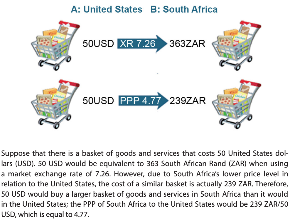
# # ℹ 161 more rows

Step 1 — exchange rates mislead. At the bank, about kr. 6.4 buy $1. But prices differ between countries: the same money buys far less in Copenhagen than in Kampala.

Step 2 — compare what money buys. Price the same basket of goods in two countries. That “exchange rate of living costs” is called purchasing power parity (PPP): what costs $1 in the US costs about kr. 6.6 in Denmark.

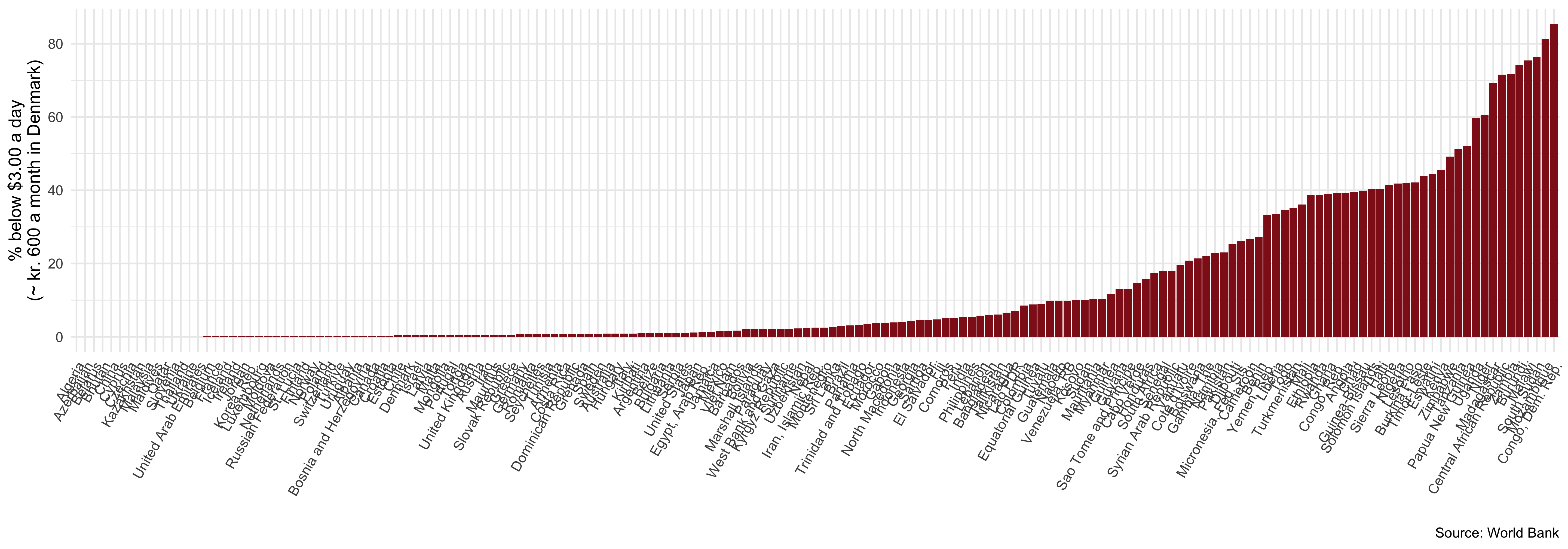
Step 3 — read the poverty line. “Below $3.00 a day (PPP)” means living on what $3 buys in the US — in Danish prices: about kr. 20 a day.

The poverty line in Danish terms: less than \(30 \times \text{kr. } 20 \approx\) kr. 600 a month — for housing, food, clothes, transport, everything.

The World Bank raised the international poverty line from $2.15 (2017 prices) to $3.00 (2021 prices) in June 2025.

Do not rush the PPP explanation — “$3.00 a day” means nothing until they can convert it. Walk the three steps, then land the Danish figure: about kr. 600 a month for housing, food, clothes, transport, everything. Let that sit for a second. A number they can feel is a number they will interpret carefully later.

Two tibbles, one analysis: relational data

If two tibbles share one or more variables, they are relational: the shared variables are the key that lets us combine them. Ours share country and year.

# Both tibbles have a `country` column with
# slightly different spellings -> keep the
# reliable key: ISO code + year
(Dat_vdem <- Dat_vdem %>% select(-country))
# # A tibble: 28,092 × 5
#    country_text_id  year civ_liberties state_own_raw state_ownership
#    <chr>           <dbl>         <dbl>         <dbl>           <dbl>
#  1 MEX              1789           0.2          -0.2             0.2
#  2 MEX              1790           0.2          -0.2             0.2
#  3 MEX              1791           0.2          -0.2             0.2
#  4 MEX              1792           0.2          -0.2             0.2
#  5 MEX              1793           0.2          -0.2             0.2
#  6 MEX              1794           0.2          -0.2             0.2
#  7 MEX              1795           0.2          -0.2             0.2
#  8 MEX              1796           0.2          -0.2             0.2
#  9 MEX              1797           0.2          -0.2             0.2
# 10 MEX              1798           0.2          -0.2             0.2
# # ℹ 28,082 more rows

Dat_poverty
# # A tibble: 171 × 4
#    country_text_id  year country    poverty
#    <chr>           <dbl> <chr>        <dbl>
#  1 ALB              2020 Albania        0.3
#  2 DZA              2011 Algeria        0  
#  3 AGO              2018 Angola        39.3
#  4 ARG              2024 Argentina      1  
#  5 ARM              2024 Armenia        0.8
#  6 AUS              2020 Australia      0.9
#  7 AUT              2023 Austria        0.5
#  8 AZE              2005 Azerbaijan     0  
#  9 BGD              2022 Bangladesh     5.9
# 10 BRB              2016 Barbados       1.7
# # ℹ 161 more rows

Join: four types

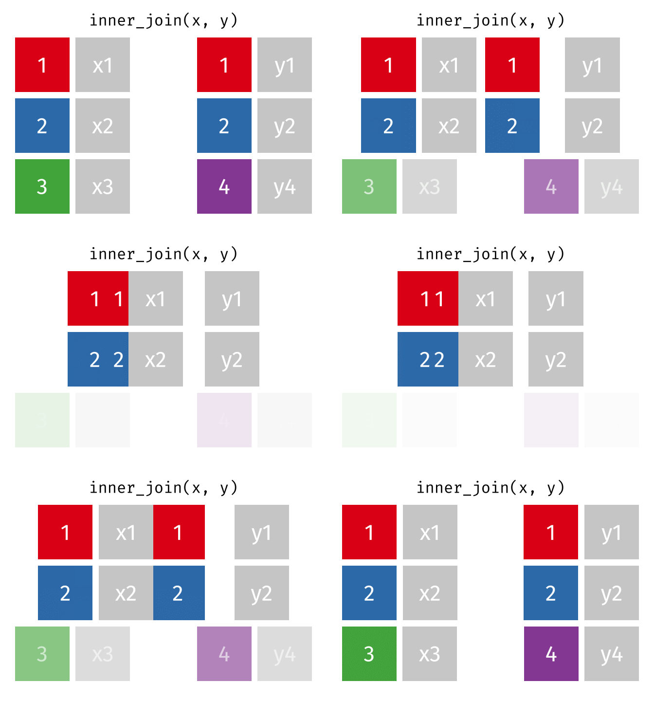
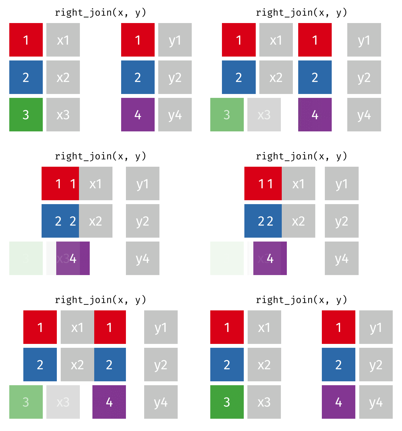
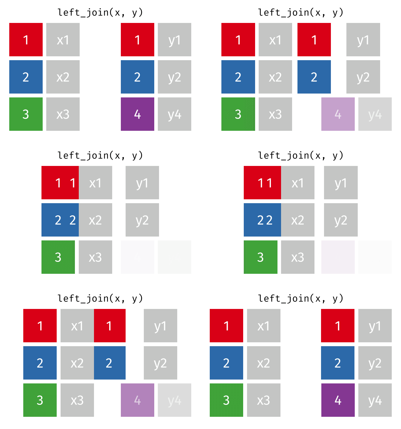
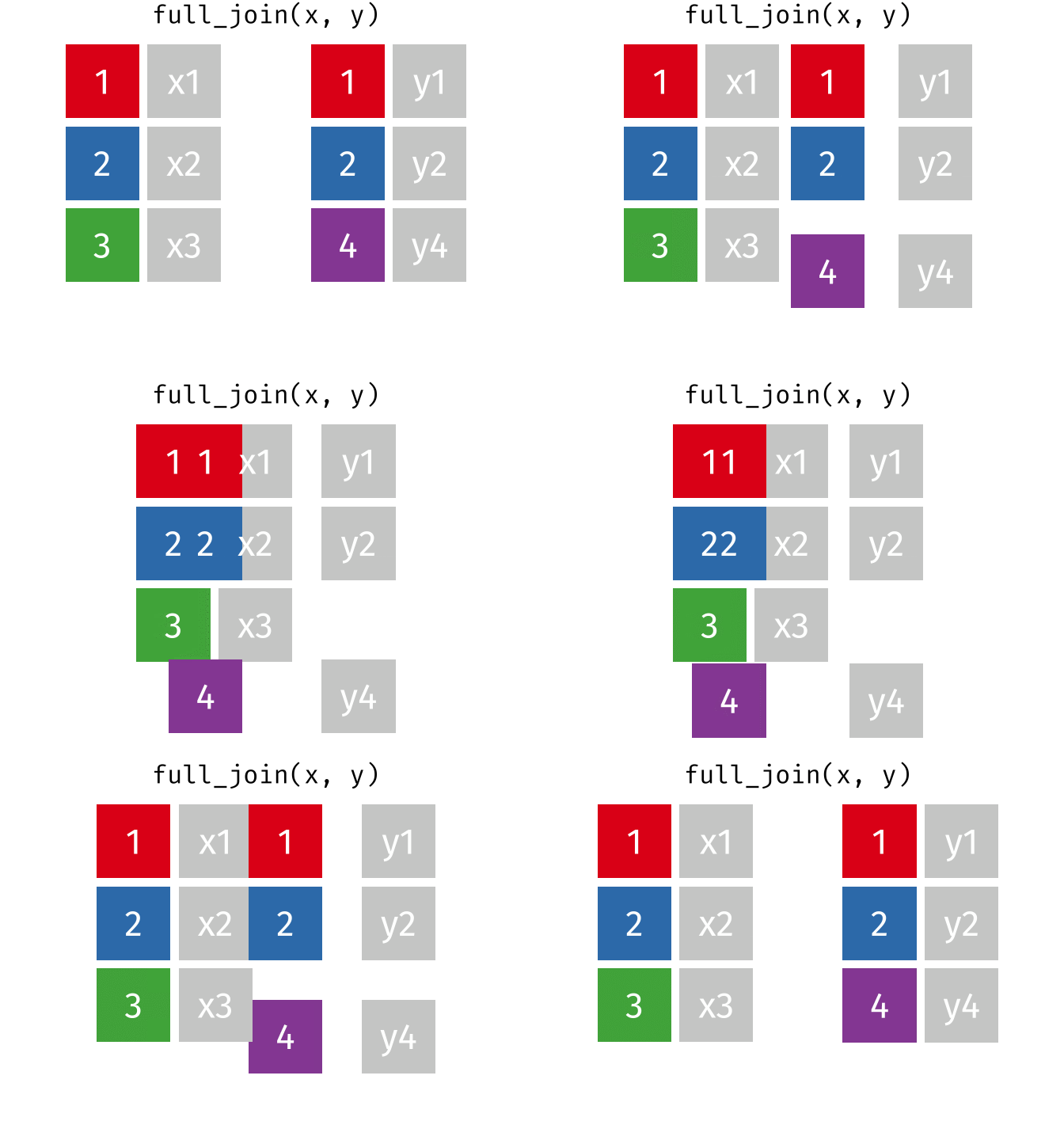
Source: Tidy Animated Verbs

Let the animations play — they explain joins better than any sentence. The only question that matters is what happens to rows that find no partner: inner keeps just the matches, left keeps everything on the left, and so on. Flag the practical trap now: inner_join() silently drops unmatched countries, so always check how many rows you started and ended with. Their exercise uses anti_join() to find exactly those.

Inner join: poverty meets civil liberties & state ownership

(Dat <- inner_join(Dat_poverty, Dat_vdem,
                   by = c("country_text_id", "year")))
# # A tibble: 161 × 7
#    country_text_id  year country    poverty civ_liberties state_own_raw state_ownership
#    <chr>           <dbl> <chr>        <dbl>         <dbl>         <dbl>           <dbl>
#  1 ALB              2020 Albania        0.3         0.914         1.57           -1.57 
#  2 DZA              2011 Algeria        0           0.575        -1.91            1.91 
#  3 AGO              2018 Angola        39.3         0.559        -0.746           0.746
#  4 ARG              2024 Argentina      1           0.844         1.39           -1.39 
#  5 ARM              2024 Armenia        0.8         0.839         1.64           -1.64 
#  6 AUS              2020 Australia      0.9         0.949         1.44           -1.44 
#  7 AUT              2023 Austria        0.5         0.937         0.479          -0.479
#  8 AZE              2005 Azerbaijan     0           0.38         -0.617           0.617
#  9 BGD              2022 Bangladesh     5.9         0.338         0.371          -0.371
# 10 BRB              2016 Barbados       1.7         0.919         0.753          -0.753
# # ℹ 151 more rows

One row per country: its most recent poverty estimate, matched to civil liberties and state ownership in that same year. All three corners of our triangle in one tibble.

Point at the key: country code and year, both needed — matching on country alone would pair a country’s poverty in one year with its politics in another. Note also why we join on the ISO code rather than the name; country names are spelled differently in every data set, which is a real and common source of silent errors.

Break

From picture to number

Part 2 of 3

Edge 1 of the triangle: state ownership and poverty — first as a picture, then as one number.

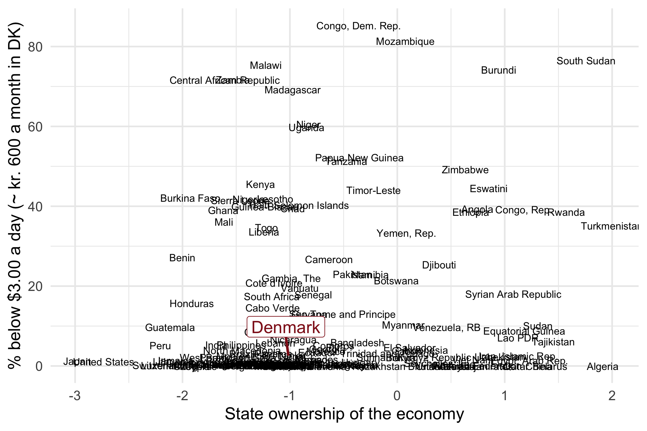
Visual inspection: the scatter plot

4 questions to ask every scatter plot:

1. What is the direction of the relationship?
2. What form does it have?
3. How much spread is there?
4. Are there outliers?

Always look before you compute — these four questions are a habit for every scatter plot in this course. Make them answer all four aloud for this plot. Find Denmark together, and ask where they expected it to sit. The eyeballed answer to edge 1 should already be “not much of a relationship”, which sets up the correlation coefficient.

Z-standardization: a common unit

• What is it?
• R code
• The picture in z-units

\[z(x) = \frac{x - \bar{x}}{\text{SD}(x)}\]

Subtract the mean: values above 0 are above average, below 0 below average.

Divide by the standard deviation: the variable’s new unit is standard deviations.

\(\rightarrow\) Intuition: how common vs. extreme is a case? And: two very different variables now share one unit.

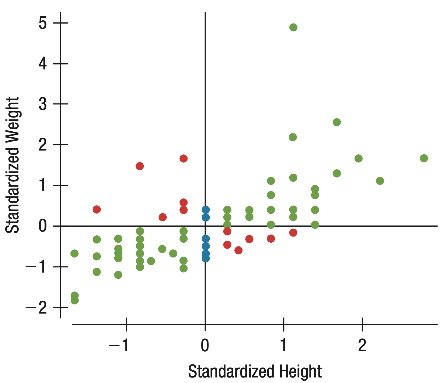
Source: Veaux, Velleman, and Bock (2021, p. 199)

(Dat <- Dat %>%
   mutate( # z-standardize both variables
     z_state_ownership = scale(state_ownership) %>% as.numeric(),
     z_poverty       = scale(poverty) %>% as.numeric()
   ))
# # A tibble: 161 × 9
#    country_text_id  year country    poverty civ_liberties state_own_raw state_ownership z_state_ownership z_poverty
#    <chr>           <dbl> <chr>        <dbl>         <dbl>         <dbl>           <dbl>             <dbl>     <dbl>
#  1 ALB              2020 Albania        0.3         0.914         1.57           -1.57            -0.893     -0.657
#  2 DZA              2011 Algeria        0           0.575        -1.91            1.91             2.58      -0.672
#  3 AGO              2018 Angola        39.3         0.559        -0.746           0.746            1.41       1.20 
#  4 ARG              2024 Argentina      1           0.844         1.39           -1.39            -0.713     -0.624
#  5 ARM              2024 Armenia        0.8         0.839         1.64           -1.64            -0.962     -0.633
#  6 AUS              2020 Australia      0.9         0.949         1.44           -1.44            -0.760     -0.629
#  7 AUT              2023 Austria        0.5         0.937         0.479          -0.479            0.194     -0.648
#  8 AZE              2005 Azerbaijan     0           0.38         -0.617           0.617            1.29      -0.672
#  9 BGD              2022 Bangladesh     5.9         0.338         0.371          -0.371            0.301     -0.390
# 10 BRB              2016 Barbados       1.7         0.919         0.753          -0.753           -0.0794    -0.590
# # ℹ 151 more rows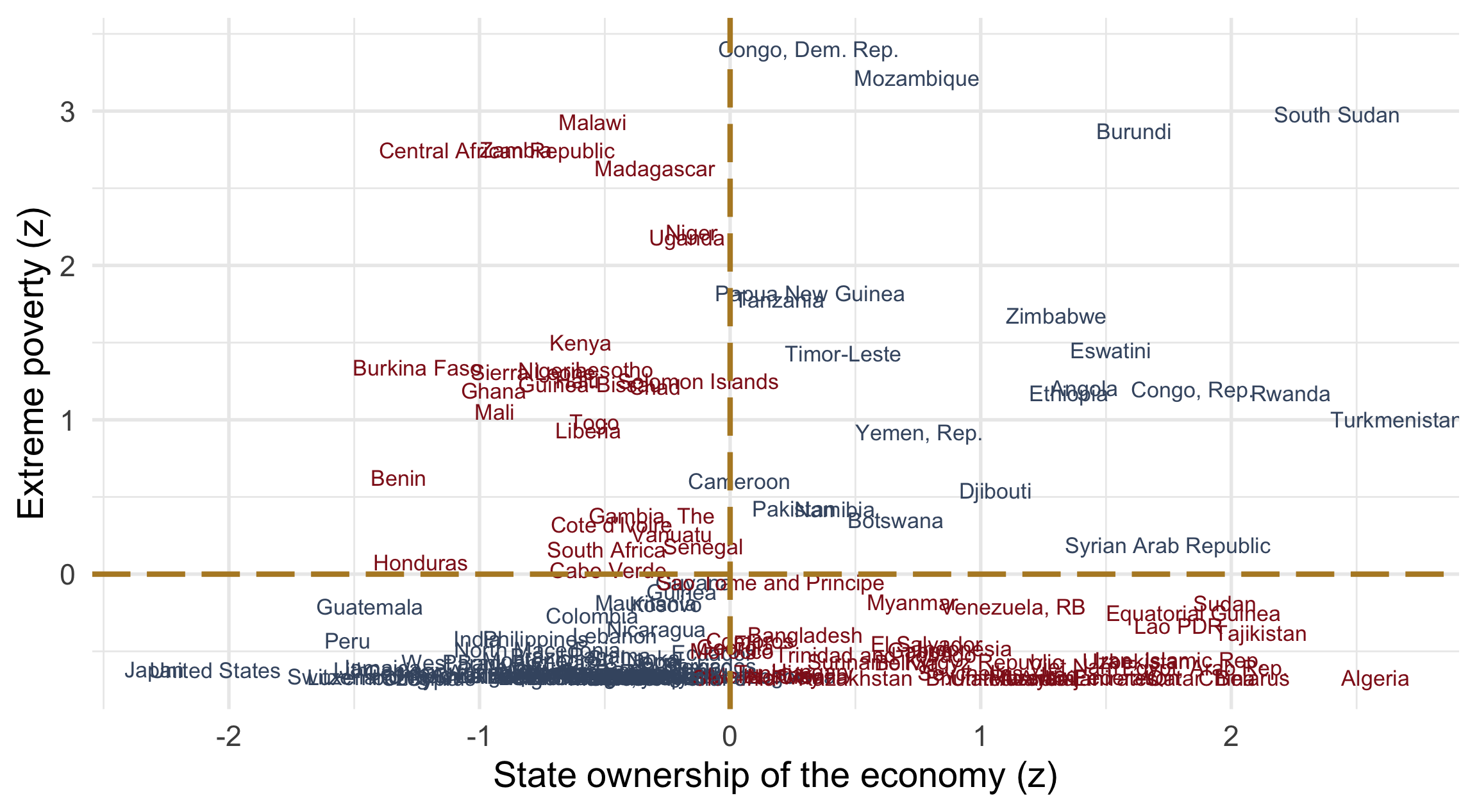

Two moves, and give each its own sentence: subtracting the mean re-centres everything on zero, dividing by the SD changes the unit to standard deviations. The payoff is that percentages and an expert-coded index now share one scale. The quadrant picture is the bridge to the next slide — countries in the blue quadrants agree in sign, those in the red disagree, and the correlation is essentially a tally of which kind dominates.

The correlation coefficient \(r_{y,x}\)

Eye-balling is not evidence. One number summarises the scatter plot:

\[r_{y,x} = \frac{\sum^{n}_{i=1}z_y \times z_x}{n-1}\]

1. \(z_y \times z_x\) is positive where a country is on the same side of both averages (blue), negative where the signs differ (red).

2. The sum \(\sum z_y z_x\) captures the general trend.

3. Dividing by \(n-1\) bounds \(r\) between \(-1\) and \(+1\).

Dat %>%
  select(poverty, state_ownership) %>%
  cor() # Estimate the correlation
#                 poverty state_ownership
# poverty           1.000           0.131
# state_ownership   0.131           1.000

Discuss: how do we interpret this \(r\)? What does it say about edge 1 of our triangle?

Essentially no linear association: state-owned economies do not have systematically less extreme poverty.

Walk the formula through the quadrant picture rather than as algebra: same-side countries contribute positive products, opposite-side ones negative, and \(r\) is essentially who wins. Then read our number — near zero, so edge 1 shows no poverty payoff. Insist on the word linear: \(r\) near zero rules out a straight-line pattern, not any relationship whatsoever.

Your turn: edge 2 of the triangle

Open exercise 1 in a new tab ↗

Break

The line: OLS regression

Part 3 of 3

From “is there a relationship?” to “how much does poverty differ with state ownership?”

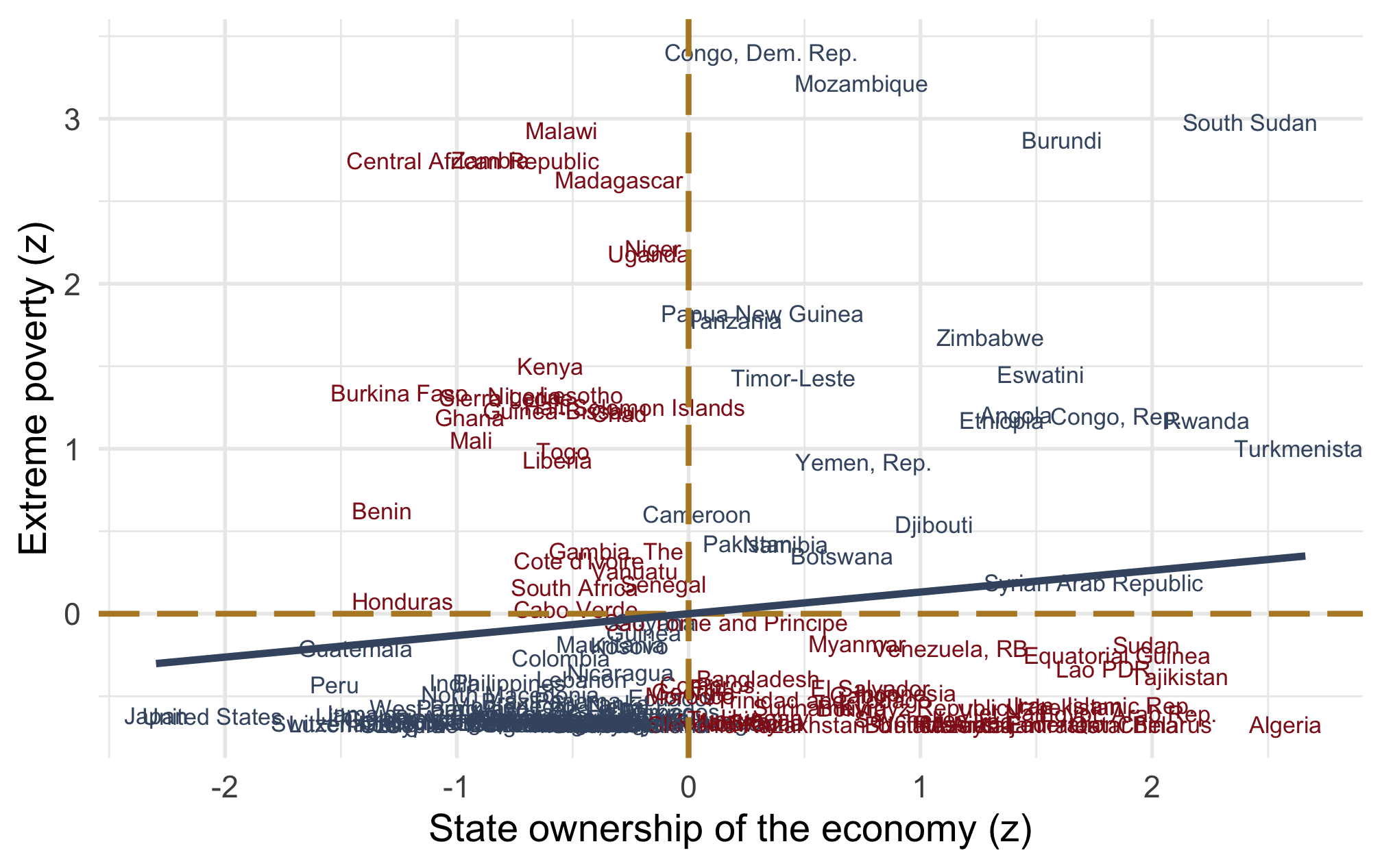
Correlation = a linear trend

How can we calculate that trend line directly?

Then we could state how much poverty differs, per unit of state ownership.

A model is a reduced representation of reality — it should capture the answer to our research question, not every data point. And it should not be driven by a few singular cases.

Linear models: two parameters

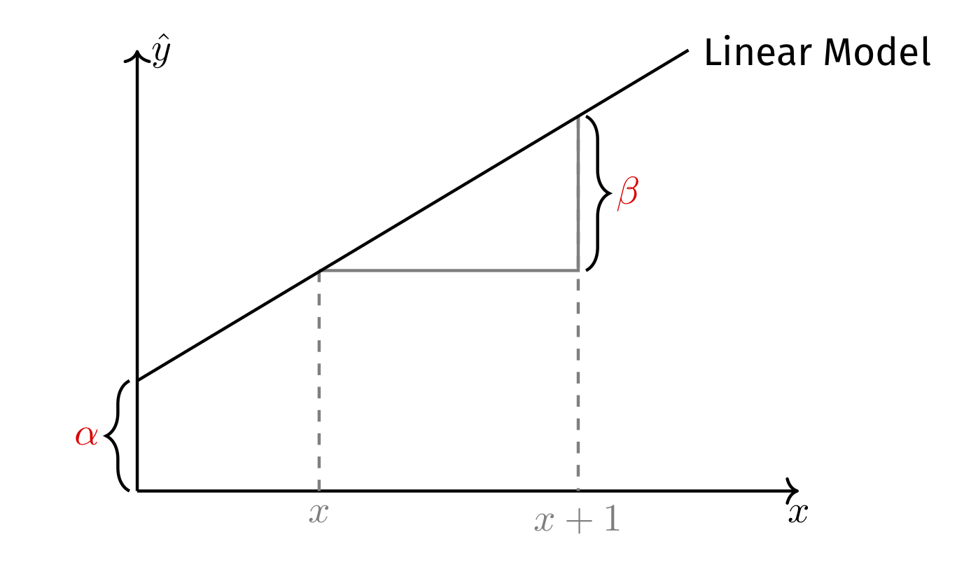
\(\alpha\), the constant/intercept: the value of \(y\) where the line crosses the Y-axis \((\hat{y} \mid x = 0)\).

\(\beta\), the slope: how \(\hat{y}\) changes when \(x\) increases by one unit.

\[\hat{y} = \alpha + \beta x\]

Two numbers fully describe a straight line: where it starts and how steeply it climbs. Keep hammering the units — \(\beta\) is “how much \(y\) changes per one unit of \(x\)”, and every interpretation they write this term should name that unit. Warn them that \(\alpha\) is only meaningful if \(x = 0\) is a real, interpretable value; here it is, because our scale is centred.

Regressing linear models from data

• Residuals, \(e\)
• The best-fitting line
• … visualized
• \(R^2\): model fit
• Regression in R
• Interpretation

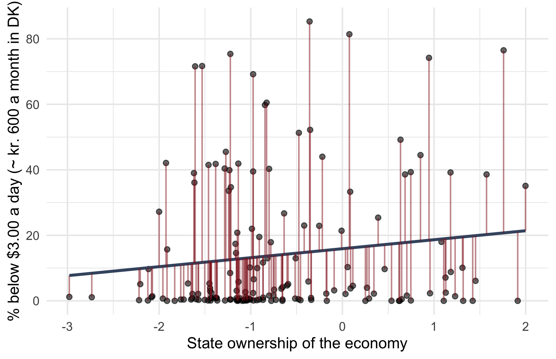
Residuals: \(e_{i} = y_{i} - \hat{y}_i\) — the differences between what the model predicts and the actual data.

For Denmark: \(e = 0.4\% - 13.2\% = -12.8\%\)

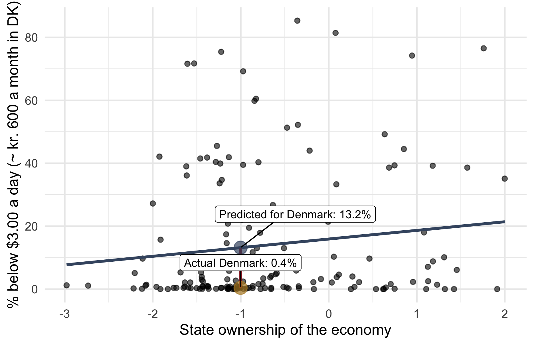
OLS finds the line that minimizes the sum of squared residuals:

\[\begin{aligned} \min \text{RSS} &= \min \sum_{i=1}^{n} e_{i}^{2} \\ &= \min \sum_{i=1}^{n} (y_{i} - (\alpha + \beta x_{i}))^{2} \end{aligned}\]

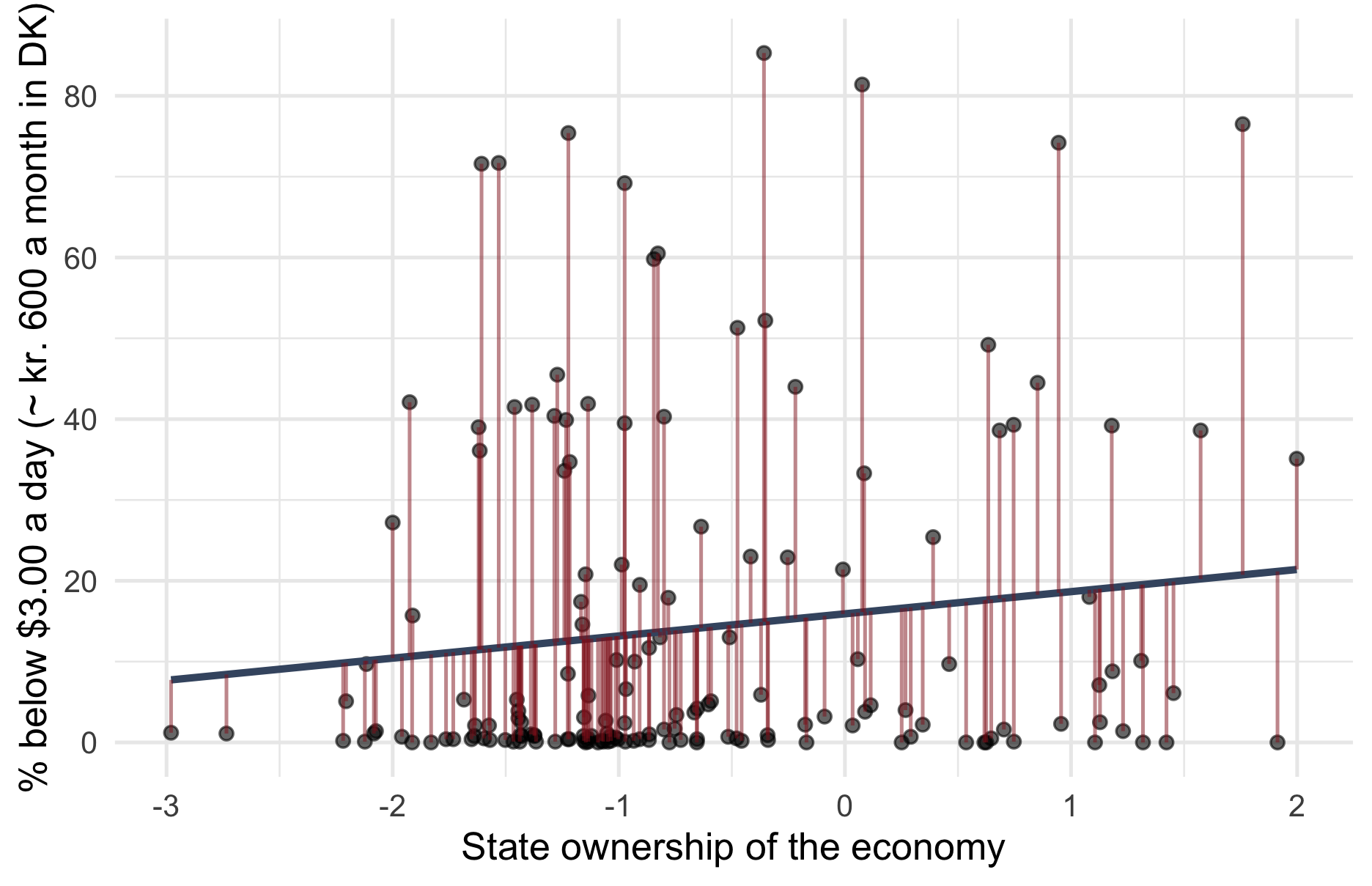
The algorithm in action: tilt and shift the line until the squared residuals cannot get any smaller.

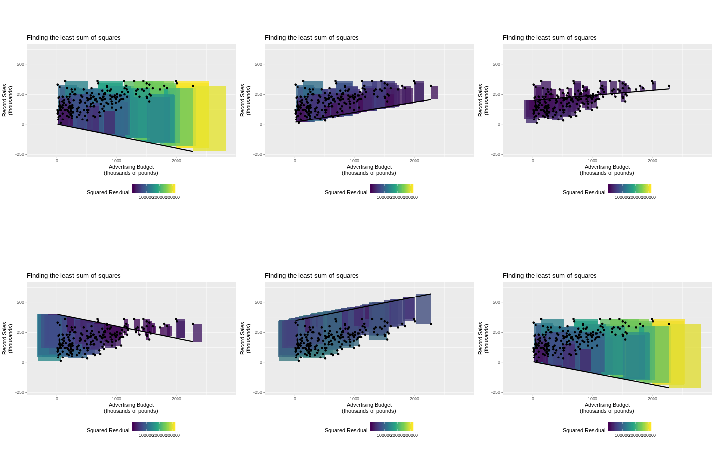
Source: aftersox on Reddit

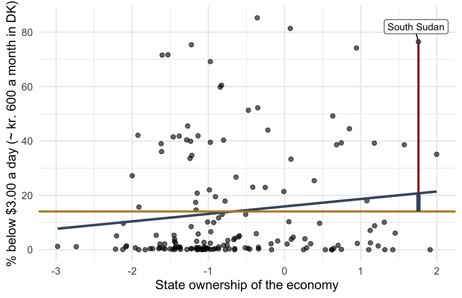
How much smaller are the residuals from our model, compared to simply predicting the average \(\bar{y}\) for everyone?

\[R^2 = \frac{\text{TSS} - \text{RSS}}{\text{TSS}}\]

with \(\text{TSS} = \sum (y_i - \bar{y})^2\) and \(\text{RSS} = \sum (y_i - \hat{y}_i)^2\).

ols <- lm_robust( # OLS with robust standard errors
  poverty ~ state_ownership,
  data = Dat
)
zols <- lm_robust( # Same, on the z-standardized variables
  z_poverty ~ z_state_ownership,
  data = Dat
)

modelsummary(
  list("OLS" = ols, "Std. OLS" = zols),
  statistic = NULL,                 # No statistical inference (yet)
  gof_map = c("nobs", "r.squared"), # Two fit statistics only
  output = "kableExtra"
)

	OLS	Std. OLS
(Intercept)	15.914	0.000
state_ownership	2.742
z_state_ownership		0.131
Num.Obs.	161	161
R2	0.017	0.017

The standardized slope of a bivariate OLS is the correlation coefficient \(r\).

A satisfying moment worth pausing on: run OLS on the z-standardised variables and the slope comes out as the correlation we computed earlier. Correlation and bivariate regression are the same fact in two costumes — regression just keeps the original units, which is what makes it interpretable.

\(\widehat{\text{Poverty}} = 15.91 + 2.74 \times \text{State ownership}\)

At the scale’s midpoint (state ownership \(= 0\)), predicted poverty is 15.91%.

With every unit more state ownership, average poverty is 2.74 percentage points higher — and \(R^2 = 0.017\): state ownership accounts for almost none of the variance in poverty across the world.

Model them the full sentence, with units, and make someone repeat it back. Then \(R^2\): state ownership explains almost none of the variation in world poverty. Say plainly that a tiny \(R^2\) is not a failed analysis — it is a finding, and here it is the answer to edge 1.

Two ways to read a regression

1. Causal

“More state ownership changes poverty by 2.74 percentage points.”

Beware: the causal reading holds only under specific conditions. Learning what those conditions are — and how to meet them — is the point of this course.

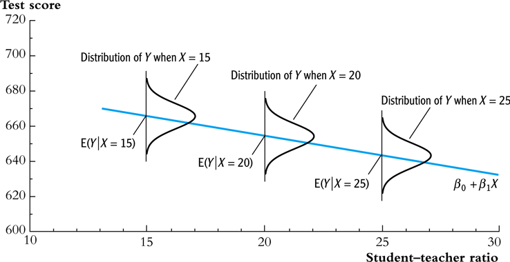
2. Descriptive: conditional means \(\bar{y} \mid x\)

“Among countries with one unit more state ownership, average poverty is 2.74 percentage points different.”

Regression as a (linear) model of averages of the outcome at different values of the predictor.

Source: Zheng Tian

The most important slide in the deck for the rest of the course. Same coefficient, two readings — one says state ownership changes poverty, the other only says countries that differ in state ownership have different average poverty. Only the second is licensed by what we did today. Give them the discipline of the descriptive phrasing, “among countries with…”, and tell them the whole course is about earning the right to the first reading.

Your turn: edge 3 — and the verdict

Open exercise 2 in a new tab ↗

The verdict: no liberty–equality trade-off

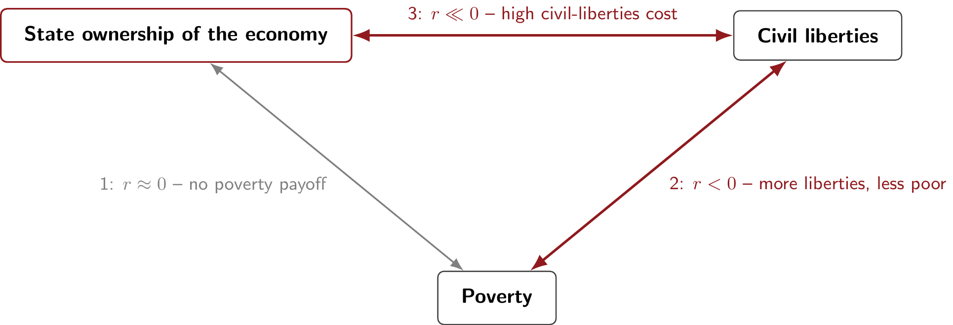
State-owned economies offer far fewer civil liberties (edge 3) and no less poverty (edge 1) — while countries with stronger civil liberties tend to have less poverty (edge 2). The premise of the trade-off does not hold in today’s data.

Careful: these are descriptive associations across countries — not yet causal effects. That distinction is where this course is headed.

Assemble the triangle with their exercise results — this is the moment the day pays off, so let them supply edges 2 and 3. The verdict: no poverty payoff, a real civil-liberties cost, and more liberties going with less poverty. The premise of the trade-off simply does not hold in these data. Then take it straight back: these are cross-country associations, and rich countries differ from poor ones in a thousand ways. That discomfort is the door into Lecture 3.

Check yourself: today’s goals

Look back at the goals from the start of the lecture. Can you tick all three?

• Download a World Bank indicator with wb_data() and join it to another data set — which variables form the key?
• Explain to your neighbour what \(r = -0.7\) means — using the word z-score at least once.
• Read \(\alpha\) and \(\beta\) from a regression table and give the descriptive interpretation of \(\beta\) — and say why the causal one needs more.

Anything feel shaky? That is what this week’s Absalon quiz and the Friday exercise class are for.

Today’s important functions

1. wb_search() / wb_data(): search and download World Bank indicators via the API.
2. inner_join(), left_join(), right_join(), full_join(): combine tibbles that share a key.
3. scale(x) %>% as.numeric(): z-standardize a variable (as.numeric() ensures a vector, not a matrix).
4. cor(): estimate the correlation coefficient.
5. estimatr::lm_robust(): linear OLS regression (with robust standard errors).
6. modelsummary(): nicely formatted tables of one or several regression models.

References

Veaux, D., Velleman, and Bock (2021). Stats: Data and Models, Global Edition. Pearson Higher Ed.