Conclusion

The whole course, on one dataset — your own

Merlin Schaeffer · Department of Sociology

2026-07-28

The goal of empirical sociology

Use data to discover patterns — and the social mechanisms that bring them about.

Fourteen weeks in two verbs: describe accurately, then explain causally. Today we put the whole toolkit on one table.

Open by naming the through-line of the entire course. Everything we did serves one of two verbs — describe a pattern well, or establish that one thing causes another. Tell them today is a map, not new material: we will walk the two halves of the course on a single, familiar dataset and see how the pieces fit. Keep it warm — it is the last lecture.

One dataset: your own quizzes

Our running example today is you: the weekly-quiz results of this class.

• mcorrect — a student’s % correct across the weeks.
• appearances — how many quizzes they completed.
• woman, Statistics — two labels we’ll build with an LLM in a moment.

Anonymised: real first names were replaced with synthetic ones. Everything numeric is exactly as it was.

Most of you did very well — the class average is 92.2% (red line).

Ground the abstractions in their own data — it lands because it is about them. Point out the average line: that single number is the simplest possible “model” of the outcome, and it is where the next slide starts. Reassure them the data are anonymised, so nobody is being singled out.

The Null model: just the average

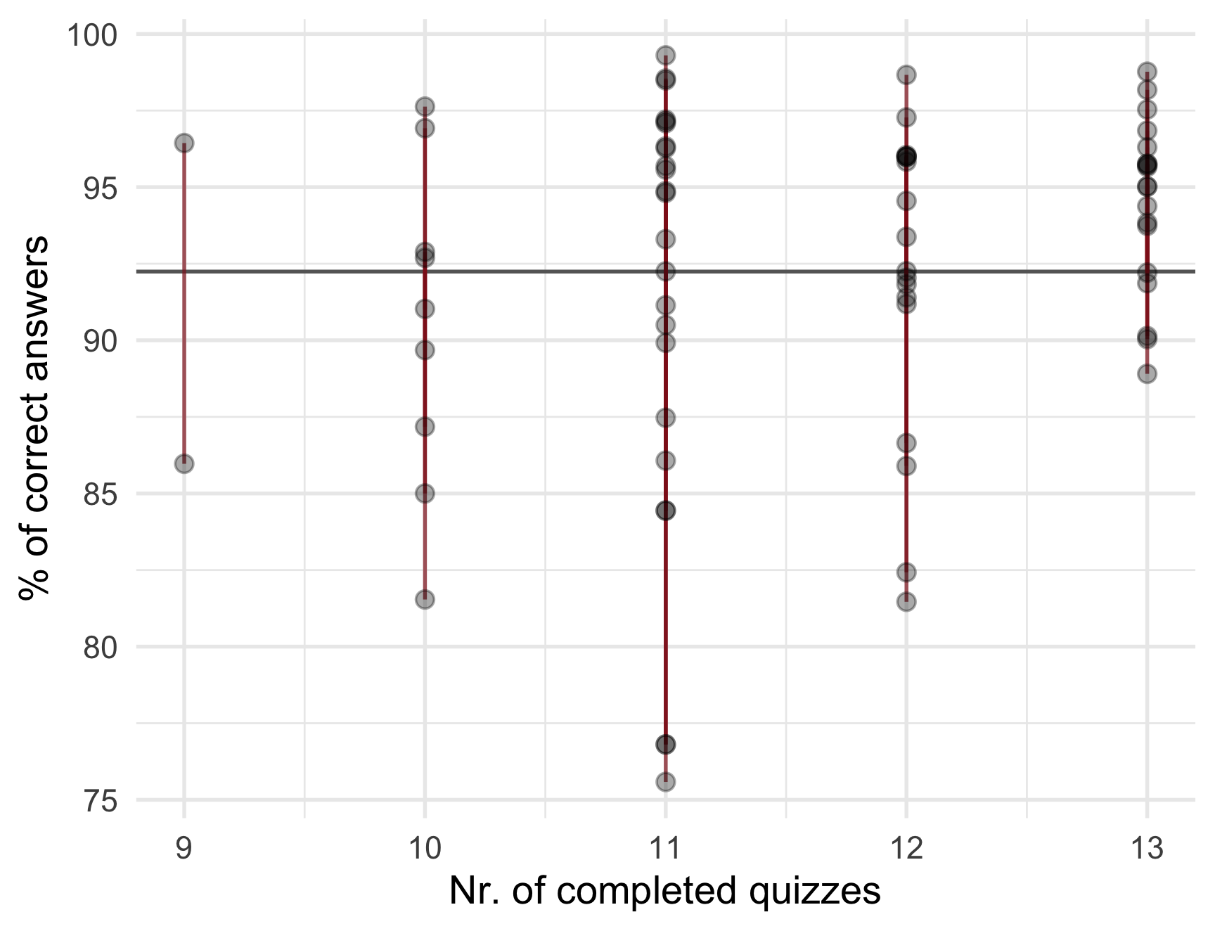
The simplest prediction of anyone’s score is the overall average \(\bar{Y}\).

It explains none of the variation between students — every red line is a full miss from the mean.

This is the baseline every model must beat. All of “describing patterns” is the effort to shrink those red lines.

The null model is the conceptual anchor of the whole descriptive half. Predict everyone with the mean and you are wrong by the red distance for each person; that total red is the variation we have not yet explained. Frame every technique that follows as a way to convert red (unexplained) into blue (explained).

OLS: a knife that cuts the variation

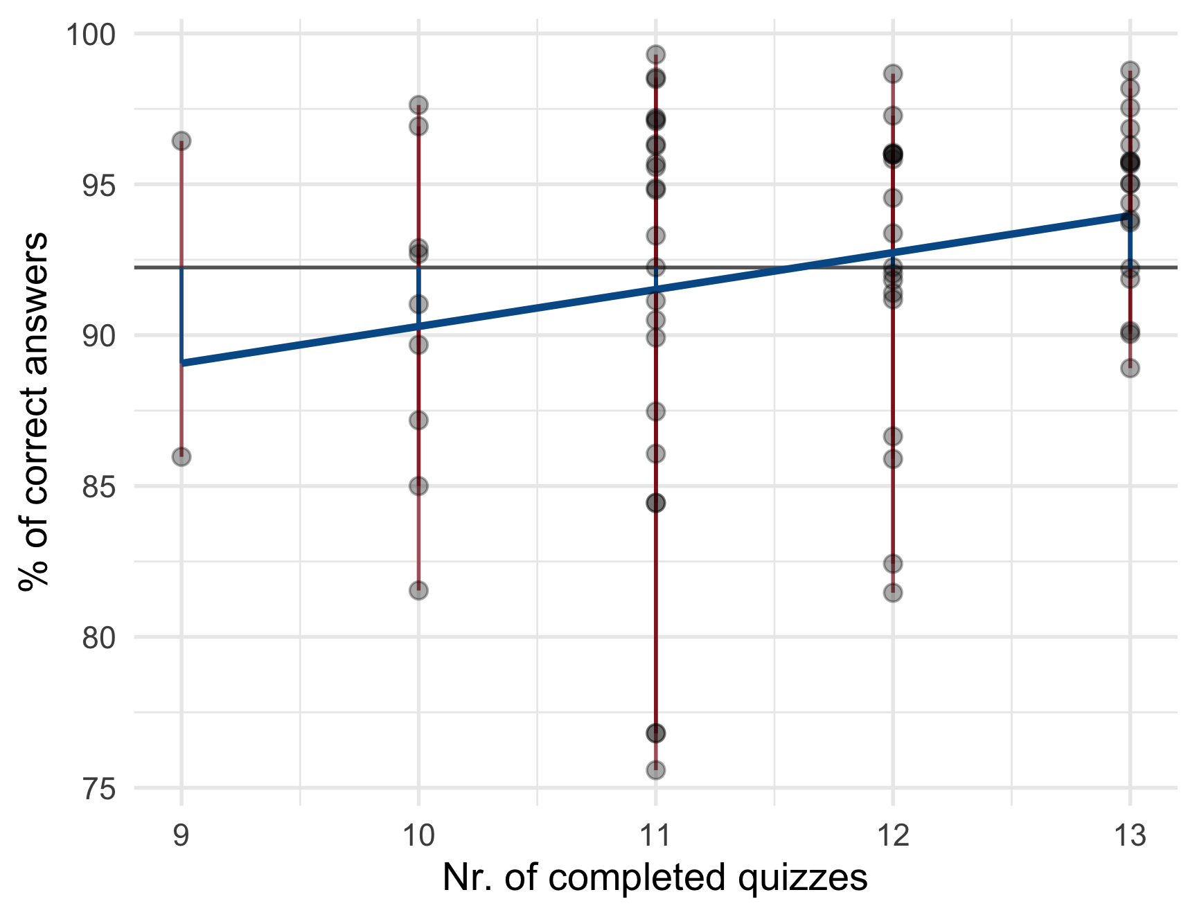
OLS fits a line by \(\min(\sum e^2)\). It splits each student’s distance from the mean into two:

• Blue — explained by the model.
• Red — residual, left unexplained.

Here the model is \[ \operatorname{mcorrect} = \alpha + \beta_{1}(\operatorname{appearances}) + \epsilon \] — score as a function of quizzes completed.

This is the single most important picture of the course, so linger. The blue segment is how far the line moved us away from the naive mean — that is explained variation. The red segment is what the line still misses. R² is simply the share of the total that turned blue. Every descriptive tool in Part 1 is a differently-shaped knife trying to turn more red into blue.

Two goals, one course

1 · Describe patterns accurately

Shrink the red, grow the blue.

1. Dummy coding — categorical predictors (L4)
2. Multiple OLS — several predictors at once (L8)
3. Interaction effects — conditional associations (L11)
4. Polynomials & transformations — non-linear shapes (L12)

2 · Identify causal mechanisms

Isolate variation in the treatment \(D\) that is as good as random.

• Assign it: RCTs (L6), natural experiments, ITT & the Wald estimator (L7)
• Find it with OLS: 2SLS (L10), control for confounders (L8/9), and regression discontinuity (L13)

Give them the map they can carry into the exam. The left column is bookkeeping on variance; the right column is a search for trustworthy variation. Stress that the whole right column exists because, in the social world, almost no variation in X is random on its own — so we either engineer randomness or hunt for a slice of it we can defend. Note RDD joined this list only last week.

Goal 1 · Describe patterns accurately

Part 1 of 2

Turn red into blue: give the model better-shaped predictors.

Categorical predictors → dummy variables

A category becomes a 0/1 dummy:

\[x = \begin{cases} 1 & \text{if the condition holds} \\ 0 & \text{otherwise} \end{cases}\]

Do women and men score differently? Let’s regress mcorrect on a gender dummy.

Beware: this cohort is 63 women vs. 9 men — the “Men” estimate rests on nine people. Read it with humility.

	% Correct
(Intercept)	93.620***
	(1.396)
Women (vs. Men)	−1.574
	(1.571)
Num.Obs.	72
R2	0.009
+ p < 0.1, * p < 0.05, ** p < 0.01, *** p < 0.001

The gap is about -1.6 points and not significant (\(p = 0.32\)) — no real gender difference here.

Recall dummy coding from Lecture 4, then use it honestly. The coefficient is the mean gap between the two groups. Two teaching moments: the estimate is not significant, so we should not claim a gender difference; and it is built on nine men, so even the point estimate is fragile. This is exactly the “read the table, and read the sample” discipline from the interaction lecture.

Where did “gender” come from? An LLM

We never asked your gender. We inferred it from first names with a zero-shot language model — the same tooling sociologists now use to code open text at scale.

Shown for transparency; the label is a prediction, not ground truth — another reason not to over-read the gap.

library(text)  # Hugging Face models from R

# Zero-shot: is a person with this name a woman?
zeroshot <- text::textZeroShot(
  sequences        = result$name,
  candidate_labels = c("woman"),
  multi_label      = FALSE,
  hypothesis_template = "A person with this name is a {}.",
  model = "alexandrainst/scandi-nli-base")

A short methods aside that students find genuinely modern: language models let us turn unstructured text — names, open answers, documents — into variables. Be candid that the gender label is a model’s guess, which compounds the earlier caution. This also sets up the joke on the next slide about what happens when you feed a model a nonsense hypothesis.

Stats skill = f(your name)?

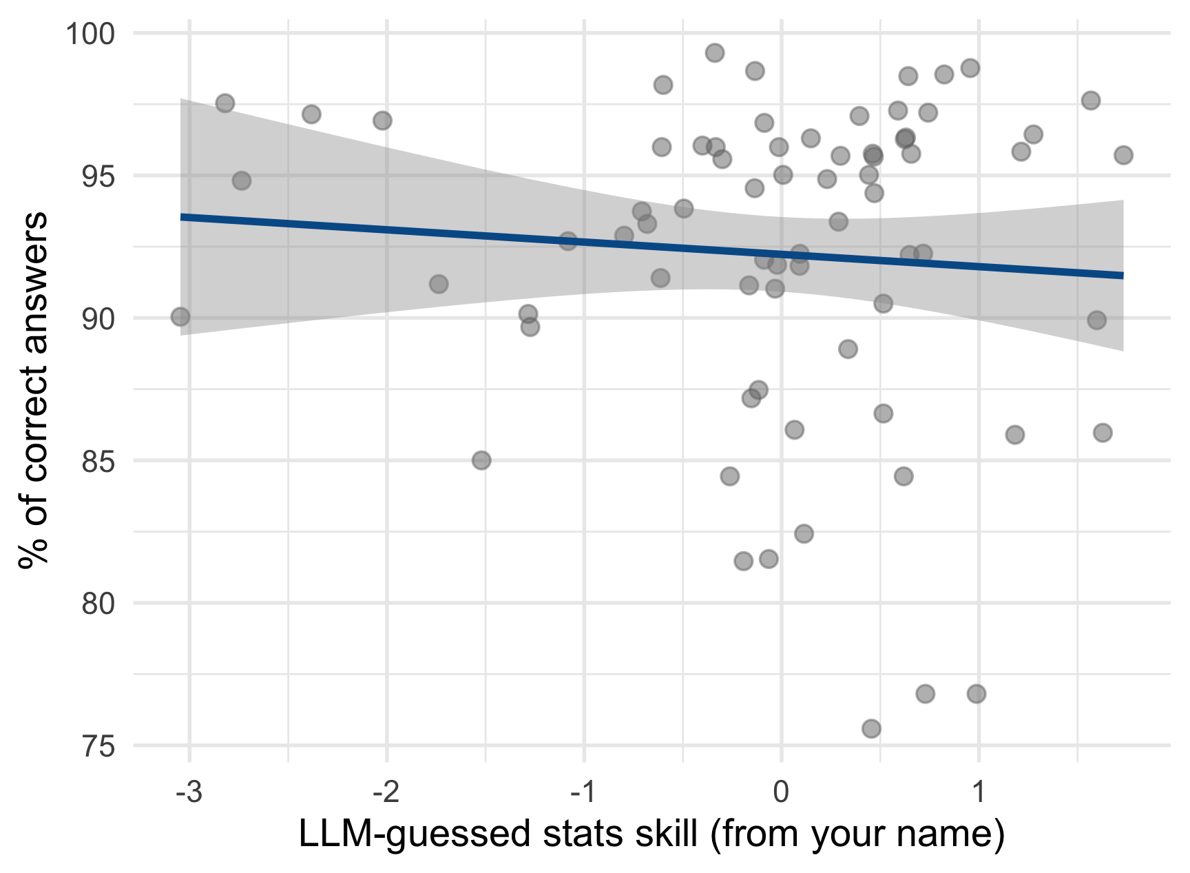
Ask the same model a silly question — “A person with this name is great at Statistics” — and it will happily return a number for every name.

Beware: a model will always answer. Slope -0.43, \(p = 0.45\), \(R^2 = 0.006\) — pure noise. Your name does not predict your stats skill.

The comic relief with a real lesson: measurement validity. The model produces a confident-looking variable that is meaningless, and a flat, non-significant line is exactly what a garbage predictor should give. Tie it back to the whole course — a coefficient is only as good as the construct behind the variable. Great note to end the “measurement” thread on before moving to multiple predictors.

Multiple OLS: several predictors at once

\[Y_i = \alpha + \beta_1 X_{1i} + \dots + \beta_k X_{ki} + \epsilon_i\]

Each slope is the association of that predictor, holding the others fixed — the Frisch–Waugh logic of Lectures 8–9.

Together, quizzes + gender + (nonsense) stats-skill explain \(R^2 = 0.092\) of the variation — a little more blue.

	% Correct
(Intercept)	79.836***
	(6.365)
Women (vs. Men)	−3.233
	(2.019)
Stats skill (LLM)	−0.826
	(0.746)
Nr. of quizzes	1.312*
	(0.564)
Num.Obs.	72
R2	0.092
+ p < 0.1, * p < 0.05, ** p < 0.01, *** p < 0.001

Recall the meaning of a multiple-regression slope: the unique association, netting out the others — the residualisation picture from Lecture 8. Note the only predictor doing real work is the number of quizzes completed; practice helps, name-noise does not. Keep it brief, it is a recap.

Interaction effects: it depends

\[Y_i = \alpha + \beta_1 X_{1i} + \beta_2 X_{2i} + \color{orange}{\beta_3\, X_{1i} X_{2i}} + \epsilon_i\]

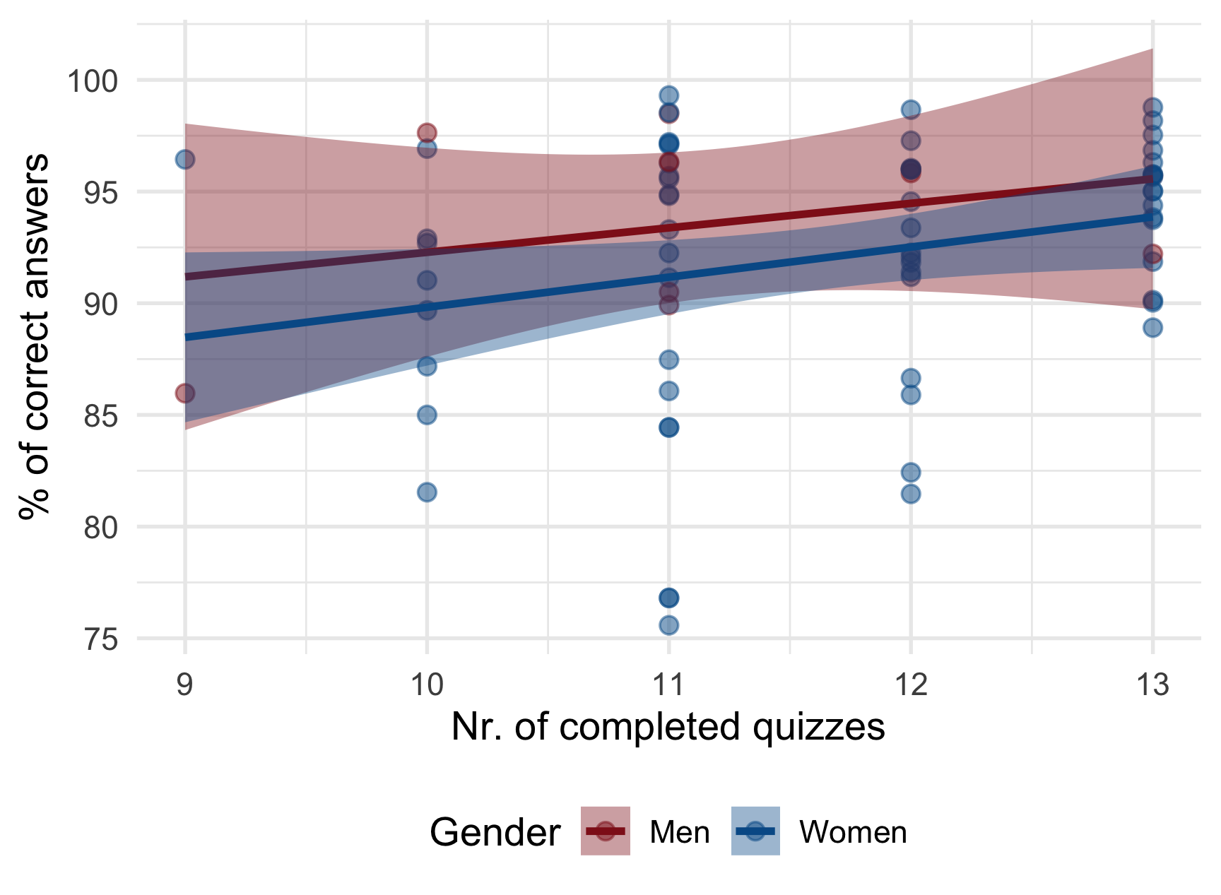
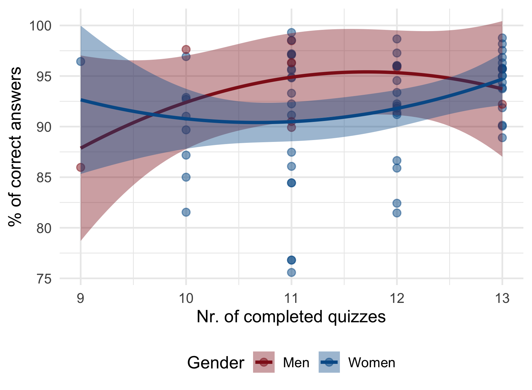
An interaction lets the slope of one predictor depend on another — the effect of practice could differ by group (L11).

Here the two slopes are nearly parallel — little evidence the quiz–score link differs by gender (and remember: nine men).

The one-line recap of interactions: the product term asks whether a slope changes across groups. Read the picture, not just the star — two near-parallel lines mean no real interaction, whatever the coefficient’s p-value says. Reinforce the humility point one more time given the tiny male group.

Polynomials: let the line bend

\[Y_i = \alpha + \beta_1 X_i + \color{orange}{\beta_2 X_i^2 + \beta_3 X_i^3} + \epsilon_i\]

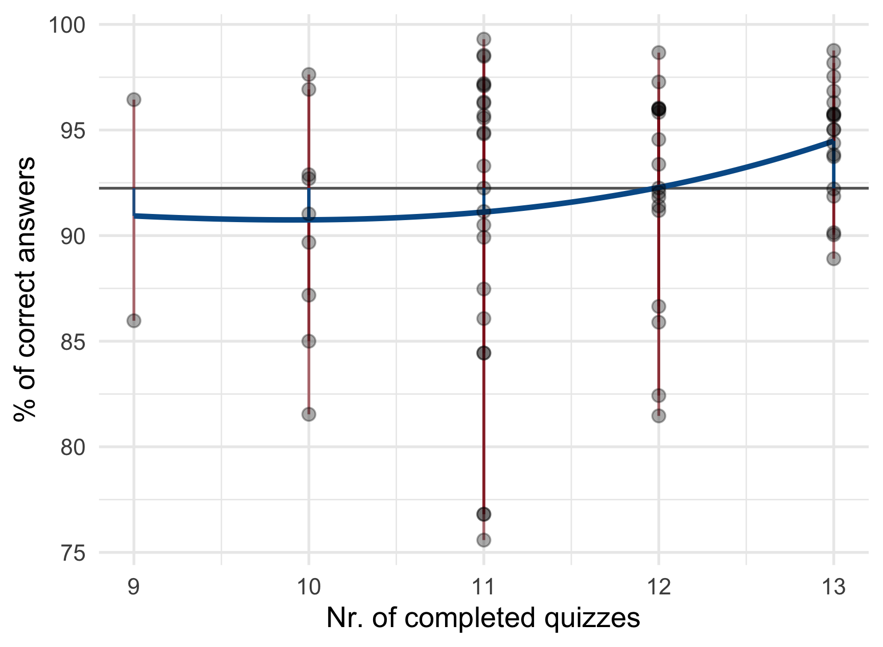
Adding powers of \(X\) bends the fit (L12) — but every extra term risks overfitting the wiggles.

A cubic nudges fit to \(R^2 = 0.068\) vs. the straight line’s \(0.058\) — barely worth the two extra terms here.

Recall the overfitting discipline from Lecture 12: use the lowest degree that captures a shape you can defend. Here the cubic barely improves on the line, so the honest choice is the line. Point at the wiggle near the edges as the visual signature of a polynomial reaching too hard.

Transformations: change the scale

\[Y_i = \alpha + \color{orange}{\beta_1 \log_2(X_i)} + \epsilon_i\]

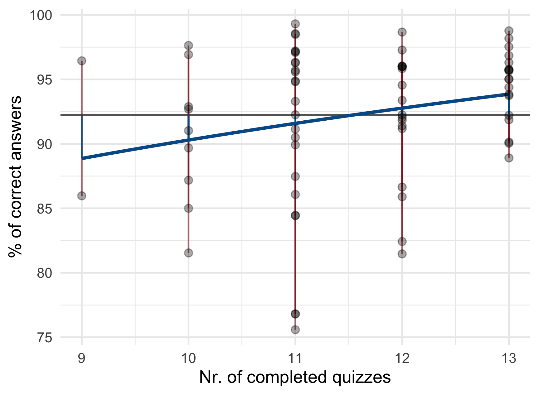
A log2 transform reads as “per doubling” (L12) — often a cleaner, one-coefficient way to capture a curve.

Each doubling of quizzes completed is worth about 9.4 points — one interpretable number.

The transformation half of Lecture 12: a log turns a curve into a straight line you can read as “per doubling”. Contrast with the polynomial — one interpretable coefficient instead of three nuisance ones. The takeaway is to match the tool to the shape you expect and can defend.

And you can combine them

\[\small Y_i = \alpha + \beta_1 X_{1i} + \beta_2 X_{2i} + \color{orange}{\beta_3 X_{1i}^2 + \beta_4 X_{1i}X_{2i} + \beta_5 X_{1i}^2 X_{2i}} + \epsilon_i\]

Dummies, curves and interactions are one toolbox — a group-specific bend is just a polynomial interacted with a dummy.

Power comes with responsibility: every term you add must earn its place, or you are fitting noise.

Synthesise Part 1: the descriptive tools all live in one formula and combine freely. But close on the warning that runs through Lectures 11 and 12 — flexibility buys fit on this sample and can cost you on the next. Describing well is disciplined, not maximal.

Goal 2 · Identify causal mechanisms

Part 2 of 2

A good description is not a cause. To claim causation we need variation in the treatment \(D\) that is as good as random.

The enemy: selection / omitted-variable bias

A raw group difference mixes the causal effect with selection bias:

\[\small \underbrace{\bar{Y}_{D=1} - \bar{Y}_{D=0}}_{\text{observed gap}} = \underbrace{\text{ATT}}_{\text{causal}} + \underbrace{\bar{Y}_{0\mid D=1} - \bar{Y}_{0\mid D=0}}_{\text{selection bias}}\]

Equivalently, an omitted confounder \(C\) bends the slope:

\[\tilde{\beta}_{Y\leftarrow D} = \beta_{Y\leftarrow D} + \underbrace{\beta_{Y\leftarrow C}\,\beta_{C\leftarrow D}}_{\text{omitted-variable bias}}\]

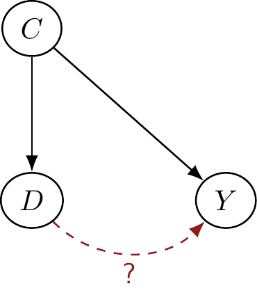
This one equation — Lectures 5 and 8 — is the reason the whole second half of the course exists.

Return to the conceptual heart of the causal half. The observed gap is contaminated whenever the treated and untreated would have differed anyway — that residual term is selection bias, and its regression twin is omitted-variable bias. Everything that follows is a strategy for killing that term: either make it zero by design, or subtract it with a control or an instrument.

Strategy A — assign \(D\) at random

Intervene so that all variation in the treatment \(D\) is random. Then the raw difference is the effect.

RCTs & natural experiments

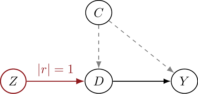
We intervene with an as-if-random \(Z\), and \(Z\) decides the treatment \(D\) perfectly \((|r| = 1)\): treatment and control differ only by chance.

• Categorical treatment → a simple \(Y = \alpha + \color{red}{\beta} I_i + \epsilon_i\) (L6).
• A natural experiment — the world does the randomising (L7) — is read the same way, if you can defend the “as-if random” arrow.

Continuous or subgroup questions still use polynomials and interactions from Part 1.

Recall Lecture 6 and 7. Randomisation cuts both dashed confounder arrows at once, which is why a bivariate model recovers the effect. A natural experiment claims the same picture but with an argument rather than a coin flip — the honesty is all in defending that the assignment really was as good as random.

When assignment is imperfect: ITT & Wald

Often \(Z\) only nudges \(D\) \((|r| < 1)\) — an offer some ignore.

• The intention-to-treat effect (the reduced form, \(\rho\)) is the effect of the offer \(Z\) on \(Y\) (L7).
• Scale it by the first stage \(\phi\) (how much \(Z\) moved \(D\)) to recover the effect of \(D\) on compliers — the Wald estimator:

\[\lambda = \frac{\rho}{\phi} = \frac{\text{reduced form}}{\text{first stage}} = \frac{\text{ITT}}{r}\]

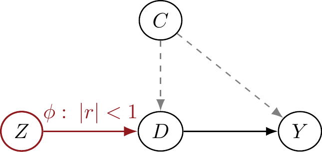
Same idea, harmonised symbols: \(\rho\) = ITT, \(\phi\) = compliance \(r\). This is exactly the L7/L10 Wald ratio.

This is the notation bridge to keep consistent: the reduced form rho is the ITT, the first stage phi is the compliance rate r, and their ratio is the Wald estimate for compliers. Say the order of operations aloud — divide the offer’s effect by how many actually complied — because students reliably invert it. It also previews why a weak first stage is dangerous: dividing by a small phi magnifies everything.

Strategy B — find random variation with OLS

Most variation in \(D\) is not random. So carve out the slice that is — and use only that.

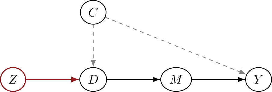
Instruments, confounders, mediators

OLS lets us split \(D\) into a trustworthy part and a contaminated part:

• Instrument \(Z\) — keep the predicted part of \(D\) driven by a random \(Z\): 2SLS (L10).
• Confounder \(C\) — throw it away by controlling: keep the part of \(D\) unrelated to \(C\) (L8/9).
• Mediator \(M\) — add it in a second step to see how much of \(D\)’s effect runs through it (L9).

Instrument vs. control — mirror images: keep the predicted values vs. keep the residuals of \(D\).

The unifying slide of the causal half, tying Lectures 8 through 10 together. Same residualisation machine, three uses: an instrument keeps the predicted part of X, a control discards the confounded part and keeps the residual, and a mediator is added deliberately to measure how much runs through it. If they can state the instrument-versus-control mirror cleanly, they have understood the second half of the course.

Regression discontinuity: the causal effect of rules

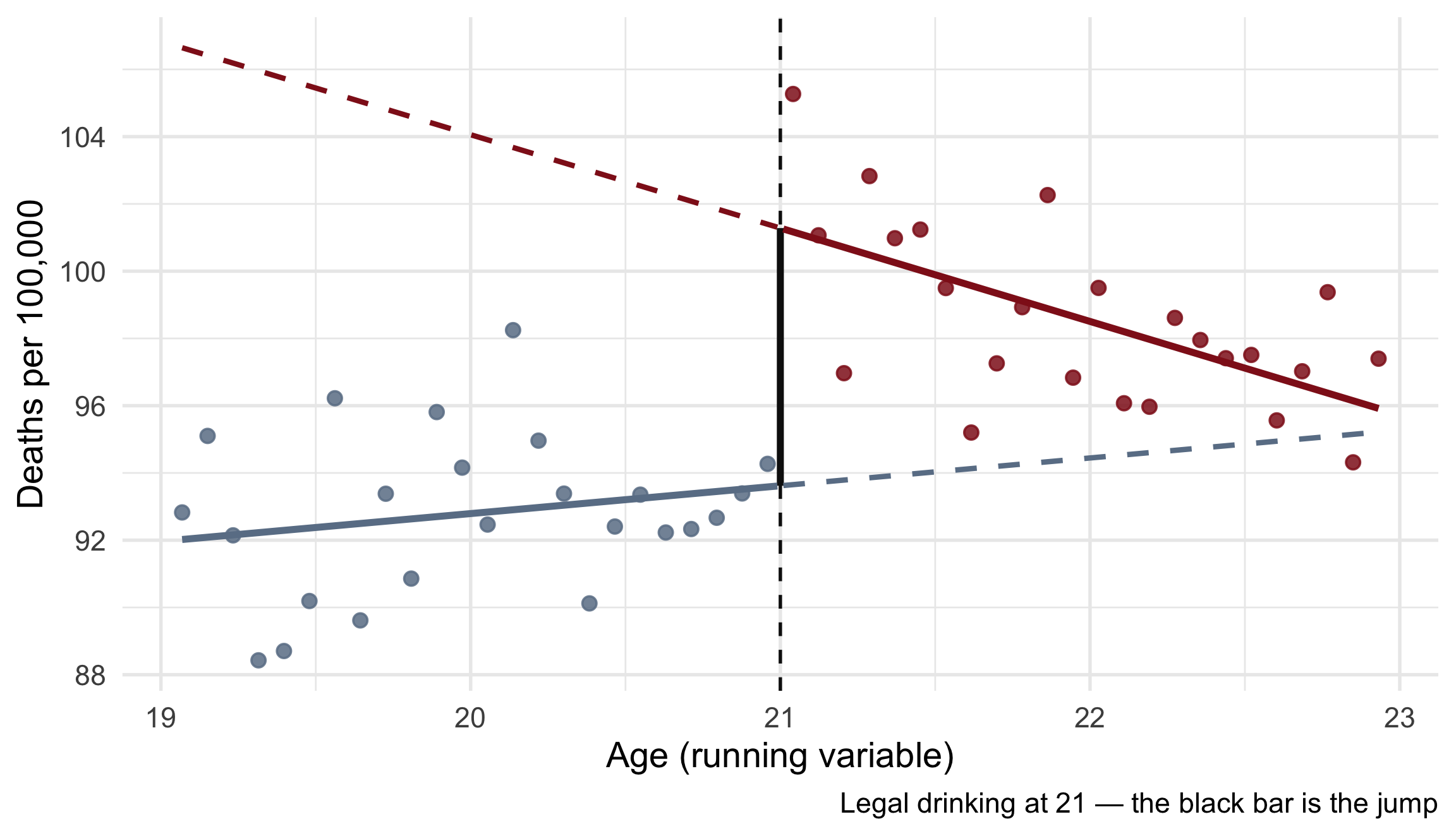
A strict rule creates a threshold on a running variable (L13). Barely below vs. barely above is as good as random — so the jump at the cutoff is the causal effect.

We fit lines on both sides using all the data, but read the gap exactly at the threshold.

Close the causal tour with last week’s design. Emphasise that RDD is the natural-experiment idea sharpened to a knife-edge: a rule, not a coin, does the splitting, and with perfect compliance the reduced-form jump is the whole effect. Point at the black bar — that vertical gap at 21 is the causal effect of legal drinking on mortality.

The whole course, in one line

Describe patterns honestly — then hunt for variation that is as good as random to explain them.

• Read and build a regression: dummies, multiple predictors, interactions, curves.
• Name selection / omitted-variable bias — and the design that defeats it.
• Tell RCT, natural experiment, IV/2SLS, control, and RDD apart, and say what each assumes.

The send-off. Compress fourteen weeks into the two verbs from the opening slide, and remind them the checklist is the exam in miniature. Thank them, and mean it — then open the floor.

Tak — spørgsmål?

Thank you for a great semester.

The weekly quiz, the Friday exercises, and this deck are your revision map for the exam.

```