Interaction Effects

When one relationship depends on another

Merlin Schaeffer · Department of Sociology

2026-07-23

By the end of today you can …

1. recognise a conditional relationship — when the association between \(Y\) and one predictor depends on another — and specify it as an interaction;

2. interpret the conditional main terms and the interaction term, and mean-centre so the main terms mean something;

3. visualise an interaction and read the conditional slopes straight off the picture.

One part per goal. Two running questions: does education reduce xenophobia the same way in Denmark and Bulgaria — and do state ownership and civil liberties interact in fighting poverty?

Everything so far has been additive: each predictor adds its own fixed amount, the same for everyone. Today that assumption breaks. Set the hook plainly — sometimes a relationship is not one number but a family of numbers, one per context. The word to keep repeating is “depends on”: the effect of X depends on Z. That phrase is the whole lecture.

Additive, so far

Everything we have built assumes predictors act additively — each adds its slice, independently of the others:

\[Y_i = \alpha + \beta_1 X_1 + \beta_2 X_2 + e_i\]

Beware: this quietly assumes the effect of \(X_1\) is the same at every value of \(X_2\). Often it is not.

Discuss: does more education reduce xenophobia by the same amount in a long-established democracy and in a post-socialist state? Should we even expect it to?

Make the hidden assumption visible, because students never notice it until you name it. A multiple regression coefficient is a single number, so it claims the effect of education is identical for a Dane and a Bulgarian, for a man and a woman, at every age. Ask whether that is plausible for the education example — most will say no, which is exactly the door into interactions.

Does education fight xenophobia everywhere?

Part 1 of 2

Education is the classic antidote to prejudice — in the West. Does the same hold in a very different context?

The research question of the day

Both Denmark and Bulgaria have seen fierce debates over immigration. In both, we can ask whether the more educated hold warmer views of immigrants.

Research question: is the link between education and xenophobia the same in Denmark and Bulgaria — or does it depend on the country?

Our outcome: agreement that “immigrants make Denmark/Bulgaria a worse place to live” — reversed so higher = more xenophobic, on a 0–10 scale.

Data: European Social Survey round 9 (2018), Danish and Bulgarian respondents.

Frame the two countries as a genuine contrast, not a throwaway: Denmark is a wealthy, long-stable democracy; Bulgaria is post-socialist, poorer, with a different history of migration. If the education effect is really about exposure and liberal values, it might travel — or it might not. That “might not” is the interaction we are chasing.

Preparation

• Packages
• Get & prepare the data

pacman::p_load(
  tidyverse,    # Data manipulation and visualization
  haven,        # Read SPSS files & handle labelled data
  estimatr,     # OLS with robust / weighted standard errors
  modelsummary  # Regression tables
)

ESS <- read_spss("../assets/ESS9e03_1.sav") %>%
  filter(cntry == "DK" | cntry == "BG") %>%        # Danes and Bulgarians
  mutate(
    cntry  = as_factor(cntry) %>% fct_relevel("Denmark"),  # Denmark = reference
    gndr   = as_factor(gndr),
    eduyrs = case_when(                             # Sensible bounds
      eduyrs < 9  ~ 9,
      eduyrs > 21 ~ 21,
      TRUE        ~ zap_labels(eduyrs)
    ),
    agea    = zap_labels(agea),
    imwbcnt = 10 - zap_labels(imwbcnt)              # Reverse: higher = more xenophobic
  ) %>%
  select(idno, cntry, pspwght, gndr, eduyrs, agea, imwbcnt) %>%
  drop_na()

Keep this quick — the only non-obvious step is reversing the outcome so that higher means more xenophobic, which makes a negative education slope read as “education reduces prejudice”. Note we keep both countries in one data set; the whole point is to compare the education slope across them.

Additive multiple OLS: one slope for everyone

• The models
• The table
• The additive plane

ols_bi   <- lm_robust(imwbcnt ~ cntry, data = ESS, weights = pspwght)
ols_add  <- lm_robust(imwbcnt ~ cntry + eduyrs, data = ESS, weights = pspwght)

modelsummary(
  list("Country only" = ols_bi, "+ education" = ols_add),
  coef_rename = c("cntryBulgaria" = "Bulgaria", "eduyrs" = "Years of education"),
  stars = TRUE, gof_map = c("nobs", "r.squared"), output = "kableExtra"
)

	Country only	+ education
(Intercept)	4.326***	4.909***
	(0.071)	(0.213)
Bulgaria	1.680***	1.635***
	(0.098)	(0.100)
Years of education		−0.043**
		(0.014)
Num.Obs.	3330	3330
R2	0.113	0.116
+ p < 0.1, * p < 0.05, ** p < 0.01, *** p < 0.001

Bulgarians are markedly more xenophobic on average, and each year of education goes with 0.043 points less xenophobia. But this forces one education slope on both countries.

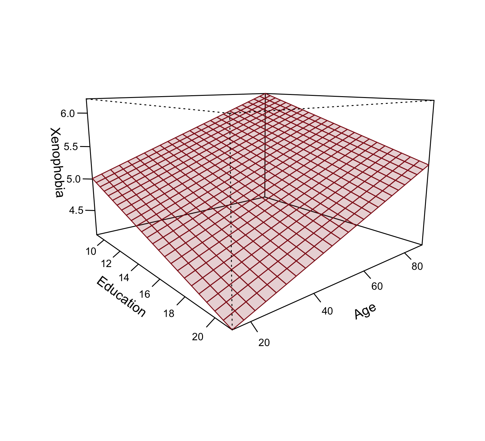
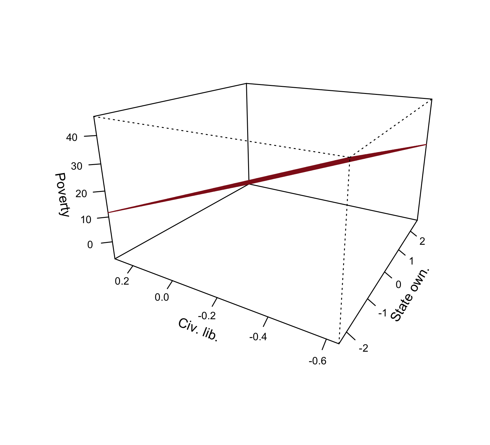
Additive = a flat, tilted plane: the education slope is the same at every age (and every country).

Two things. First, the additive model already tells a story — Bulgarians more xenophobic, education associated with less. Second, and this is the setup for everything: this model forces a single education slope on both countries. Point at the plane and say it is flat and rigid — tilt it however you like, the slope in one direction never changes as you move along the other. An interaction is what lets the plane bend.

But what if the relationship is conditional?

Two predictors interact when the association between \(Y\) and one of them depends on the value of the other.

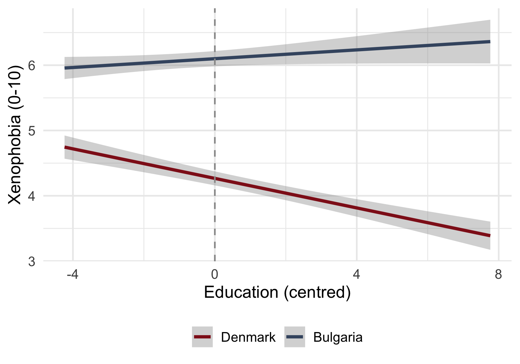
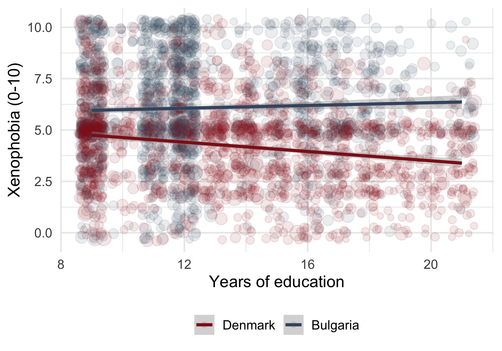
Look at the two clouds separately:

• In Denmark, education slopes clearly downward — the educated are less xenophobic.
• In Bulgaria, the line is nearly flat — education barely moves xenophobia.

\(\rightarrow\) The education effect depends on the country. That is an interaction.

Let them read the picture before you give them the definition — the two slopes are visibly different, and that is the interaction, made concrete. Say the definition twice, slowly: an interaction is when the effect of one variable depends on the level of another. Then note it is symmetric, which trips people up: “education depends on country” and “the country gap depends on education” are the same statement seen from two sides.

Specify it as multiplicative

We add the product of the two predictors:

\[Y_i = \alpha + \beta_1 X_1 + \beta_2 X_2 + \color{#901A1E}{\beta_3 (X_1 \times X_2)} + e_i\]

# The * asks R for both main terms AND their product
ols_int <- lm_robust(imwbcnt ~ cntry * eduyrs,
                     data = ESS, weights = pspwght)

cntry * eduyrs is shorthand: R adds cntry, eduyrs, and cntry:eduyrs, the interaction term.

	Additive	 Interaction
(Intercept)	4.909***	5.873***
	(0.213)	(0.279)
Bulgaria	1.635***	−0.375
	(0.100)	(0.385)
Education	−0.043**	−0.113***
	(0.014)	(0.019)
Bulgaria × Education		0.153***
		(0.027)
Num.Obs.	3330	3330
R2	0.116	0.127
+ p < 0.1, * p < 0.05, ** p < 0.01, *** p < 0.001

OLS handles a multiplicative idea by adding one column — the product of the two variables. The conditional relationship is linearised.

The mechanics are trivial and worth saying so: an interaction is just one more predictor, the two variables multiplied together. * is R’s shorthand that also remembers to include the main terms. The deeper point is the green box — regression is fundamentally additive, and it accommodates a “depends on” relationship by literally adding a product column. Do not interpret the coefficients yet; that is the next, harder slide.

The trap: what do the main terms mean now?

	 Interaction
(Intercept)	5.873***
	(0.279)
Bulgaria	−0.375
	(0.385)
Education	−0.113***
	(0.019)
Bulgaria × Education	0.153***
	(0.027)
Num.Obs.	3330
+ p < 0.1, * p < 0.05, ** p < 0.01, *** p < 0.001

Once you add the product, each main term is conditional — it holds only where the other variable is zero:

\[\beta_{\text{Education}} \;\big|\; \text{Bulgaria} = 0 \quad(\text{i.e. in Denmark})\] \[\beta_{\text{Bulgaria}} \;\big|\; \text{Education} = 0\]

Beware: the “Bulgaria” coefficient is now the country gap at zero years of education — a person who does not exist. No wonder it looks strange.

This is where students fall off, so slow right down. The moment you add the product, the two main terms stop being averages and become conditional — each is the effect of one variable at the point where the other equals zero. The education coefficient is the Danish slope, because Bulgaria = 0 means Denmark. The country coefficient is the gap at zero years of education — nobody in the sample. That absurdity is not a bug; it is a signal that we should move zero somewhere meaningful.

The fix: mean-centre

Shift education so that zero = the average:

ESS <- ESS %>%
  mutate(mc_eduyrs = eduyrs - mean(eduyrs))

ols_intc <- lm_robust(imwbcnt ~ cntry * mc_eduyrs,
                      data = ESS, weights = pspwght)

Now Education = 0 means “a person with average schooling” — a real, typical case. The interaction term is unchanged; only the main terms move to where we can read them.

	Raw	Mean-centred
(Intercept)	5.873***	4.378***
	(0.279)	(0.072)
Bulgaria	−0.375	1.650***
	(0.385)	(0.099)
Education	−0.113***
	(0.019)
Bulgaria × Educ	0.153***	0.153***
	(0.027)	(0.027)
Education (centred)		−0.113***
		(0.019)
Num.Obs.	3330	3330
+ p < 0.1, * p < 0.05, ** p < 0.01, *** p < 0.001

The Bulgaria gap becomes the gap at average education — sensible, and significant.

The cure is one line, and the effect is dramatic — watch the country coefficient move from a strange negative number to the substantively meaningful gap at average education. Stress what does not change: the interaction term is identical, because centring only relocates zero, it does not alter how the slopes differ. Tell them to centre continuous variables involved in interactions by default; it is almost always the right move.

Reading the interaction term

The interaction term (0.153) reads two ways:

1. It is how much the education slope changes from Denmark to Bulgaria: \[\underbrace{-0.113}_{\text{DK slope}} + \underbrace{0.153}_{\text{interaction}} = \underbrace{0.04}_{\text{BG slope}}\]

2. It is how much the country gap changes with each year of education.

Education fights xenophobia in Denmark (slope -0.113) but is essentially flat in Bulgaria (slope 0.04).

Return to the symmetry, now with numbers. The single interaction coefficient answers two questions at once: how the education slope differs between countries, and how the country gap grows with education. Walk the little sum — the Danish slope plus the interaction equals the Bulgarian slope. Then the substantive headline: the liberal-education story holds in Denmark and essentially fails in Bulgaria. That is a finding, and it is exactly what a single additive slope would have hidden.

A second example: education × gender

• The picture
• The model
• Read it

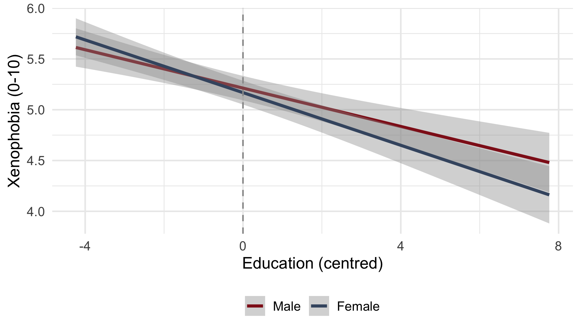
ols_eg <- lm_robust(imwbcnt ~ mc_eduyrs * gndr,
                    data = ESS, weights = pspwght)

modelsummary(list("Xenophobia" = ols_eg),
             coef_rename = c("mc_eduyrs" = "Education (centred)",
                             "gndrFemale" = "Female",
                             "mc_eduyrs:gndrFemale" = "Education × Female"),
             stars = TRUE, gof_map = c("nobs"), output = "kableExtra")

	 Xenophobia
(Intercept)	5.278***
	(0.075)
Education (centred)	−0.060**
	(0.021)
Female	−0.097
	(0.102)
Education × Female	−0.037
	(0.029)
Num.Obs.	3330
+ p < 0.1, * p < 0.05, ** p < 0.01, *** p < 0.001

Discuss: interpret the Female coefficient. At what value of education does it hold — and is that why it may look small?

A second worked case cements the pattern, now with two continuous-looking main terms plus their product. Push them to state the conditions out loud: the education slope is “among men”, the gender gap is “at average education”. Whether the slopes differ significantly matters less here than that they can say what each number is conditional on. That is the transferable skill.

Break

Your turn: exercise 1

You test whether the Bali terror-attack effect was the same across ten countries — a treatment × country interaction on Legewie’s data.

Open exercise 1 in a new tab ↗

Two continuous predictors

Part 2 of 2

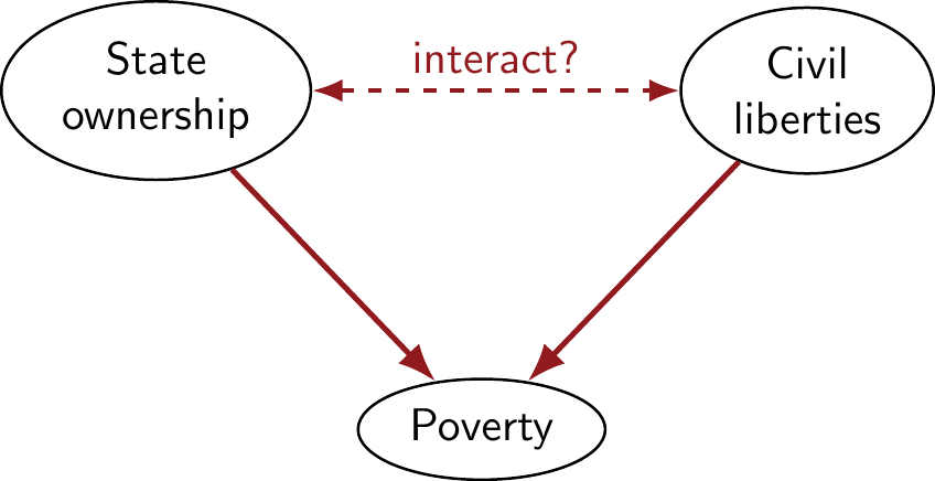
Back to the state-ownership triangle from Lectures 2 and 9 — but now the two arms of the triangle interact.

Revised research question

In Lecture 9 we asked whether civil liberties confound or mediate the link between state ownership of the economy and poverty.

Today we ask something sharper:

Research question: does state ownership fight poverty differently depending on the level of civil liberties — strong under one, weak under the other?

Tie this explicitly to Lecture 9 so it reads as one continuing story, not a new topic. There we treated civil liberties as a possible confounder or mediator; here we ask whether the two predictors interact — whether state ownership’s effect on poverty is one thing under liberal rule and another under autocracy. Same three variables, a new and more demanding question.

Build the triangle data

pacman::p_load(tidyverse, estimatr, vdemdata, wbstats, modelsummary)

# V-Dem: civil liberties, and state ownership (reversed so higher = more)
Dat_vdem <- vdem %>%
  as_tibble() %>%
  select(country_text_id, year,
         civ_liberties = v2xcl_rol,
         state_own_raw = v2clstown) %>%
  mutate(state_ownership = -state_own_raw)

# World Bank: extreme poverty (< $3.00 a day). Live, with cached fallback.
Dat_pov <- tryCatch(
  wb_data("SI.POV.DDAY", start_date = 1972, end_date = 2025),
  error = function(e) readRDS("data/wb_poverty_raw.rds")
) %>%
  rename(poverty = SI.POV.DDAY, year = date, country_text_id = iso3c) %>%
  select(country_text_id, year, country, poverty) %>%
  drop_na(poverty) %>%
  group_by(country) %>% filter(year == max(year)) %>% ungroup()

Dat <- inner_join(Dat_pov, Dat_vdem, by = c("country_text_id", "year")) %>%
  drop_na(poverty, state_ownership, civ_liberties) %>%
  mutate(                                # Mean-centre BOTH, ready for the interaction
    mc_state = state_ownership - mean(state_ownership),
    mc_civ   = civ_liberties  - mean(civ_liberties)
  )

This is the exact L2/L9 pipeline — live World Bank data with a cached fallback so the render never dies on an API outage, the reversed V-Dem state-ownership measure, and the $3.00 poverty line. The new step is at the bottom: mean-centre both continuous predictors before interacting them, for the same reason as in Part 1 — so the main terms read at the average, not at an impossible zero.

Additive first: one flat plane

ols_add2 <- lm_robust(poverty ~ mc_state + mc_civ,
                      data = Dat)

modelsummary(list("Poverty" = ols_add2),
             coef_rename = c("mc_state" = "State ownership",
                             "mc_civ" = "Civil liberties"),
             stars = TRUE, gof_map = c("nobs", "r.squared"),
             output = "kableExtra")

The additive state-ownership slope is -3.78 — the very number from Lecture 9. One flat plane, one slope for all.

Anchor on the continuity: the additive slope is −3.78, exactly Lecture 9’s number, so nothing has changed yet. The plane is flat and tilted — as you slide along the civil-liberties axis, the tilt in the state-ownership direction never changes. That rigidity is precisely the assumption we are about to test. Keep the plane on screen; the next one bends.

Now let the plane bend

ols_int2 <- lm_robust(poverty ~ mc_state * mc_civ,
                      data = Dat)

modelsummary(
  list("Additive" = ols_add2, "Interaction" = ols_int2),
  coef_rename = c("mc_state" = "State ownership",
                  "mc_civ" = "Civil liberties",
                  "mc_state:mc_civ" = "State own. × Civ. lib."),
  stars = TRUE, gof_map = c("nobs", "r.squared"),
  output = "kableExtra"
)

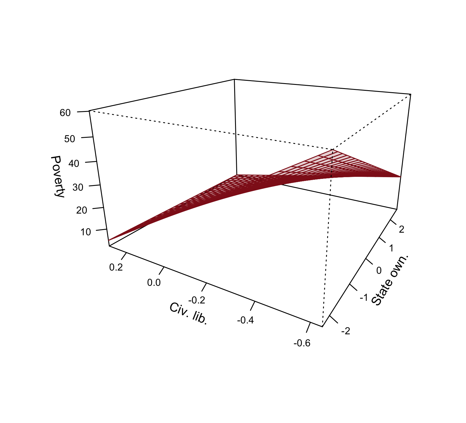
An interaction implies non-linearity: the surface is no longer flat. The fitted effect of state ownership now twists as civil liberties rise — though whether that twist is real is a question the table, not the plane, must answer.

Here is the intuition the 3D view is for: adding the product warps the plane into a twisted surface — the slope in one direction genuinely changes as you move along the other. Say the slightly surprising thing out loud: an interaction between two continuous variables is a form of non-linearity, a saddle. The 3D plane is great for feeling that, and hopeless for reading exact numbers — which is why the next slide flattens it into lines.

Read it as lines, not a surface

• Plot
• R code

# 1. One standard deviation of the moderator (civil liberties)
sd_c <- sd(Dat$mc_civ)

# 2. A grid: many state-ownership values, at THREE civil-liberties levels
grid <- expand.grid(
  mc_state = seq(min(Dat$mc_state), max(Dat$mc_state), length.out = 50),
  mc_civ   = c(-sd_c, 0, sd_c)             # low, average, high
)

# 3. Predict poverty from the interaction model on that grid
grid$poverty   <- predict(ols_int2, newdata = grid)
grid$Liberties <- factor(grid$mc_civ,
  labels = c("Low (autocratic)", "Average", "High (liberal)"))

# 4. One line per civil-liberties level
ggplot(grid, aes(x = mc_state, y = poverty, color = Liberties)) +
  geom_line(linewidth = 1.1) +
  scale_color_manual(values = c("#901A1E", "#b5892c", "#425570")) +
  labs(x = "State ownership (centred)",
       y = "Predicted % below $3.00 a day",
       color = "Civil liberties") +
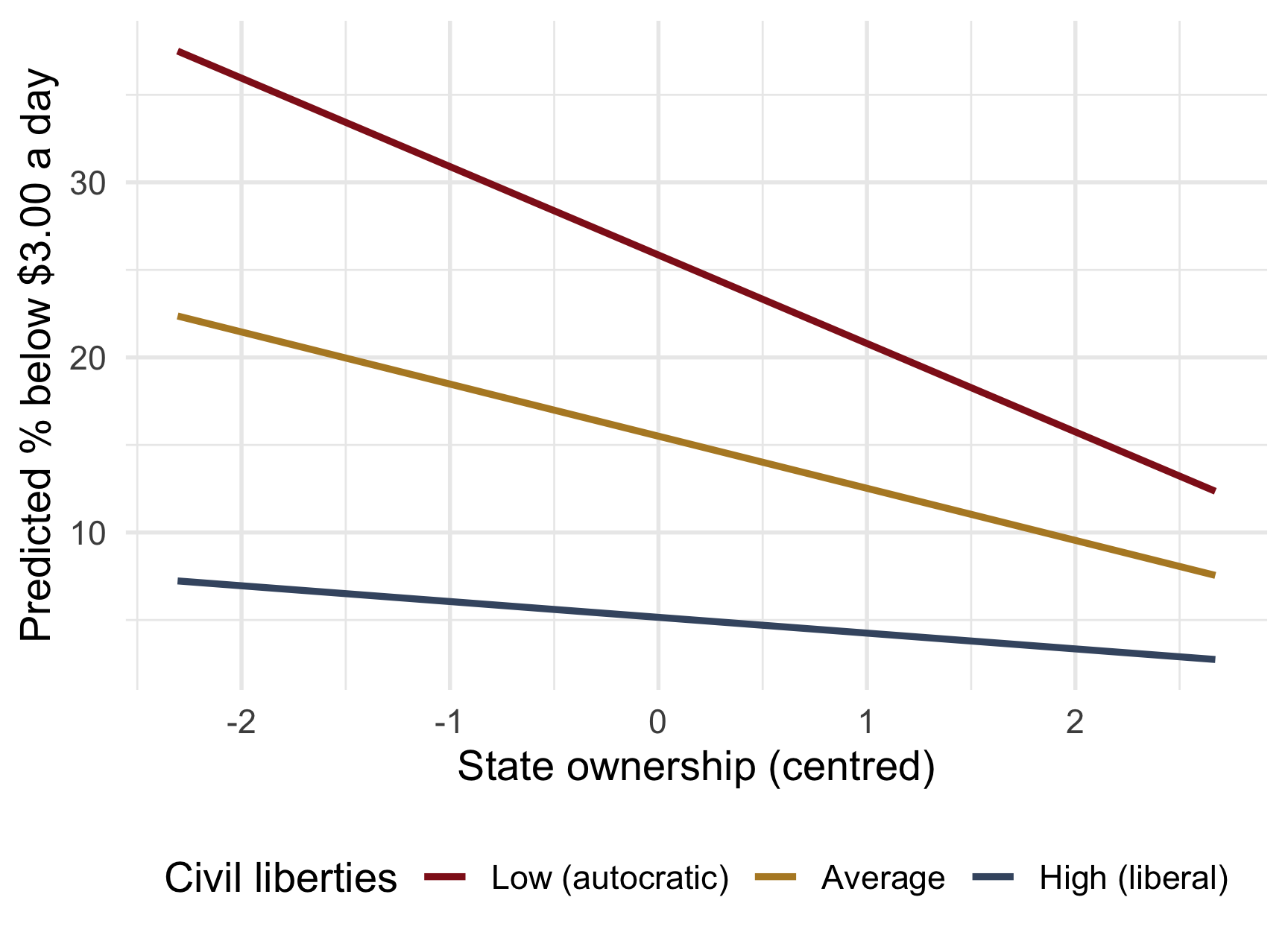
  theme_minimal(base_size = 14) + theme(legend.position = "bottom")

The same model, drawn as the state-ownership slope at three levels of civil liberties:

• Low civil liberties (autocratic): slope -5.05 — state ownership appears to go with less poverty.
• Average: slope -2.98.
• High civil liberties (liberal): slope -0.9 — state ownership appears to barely matter.

Beware — read the table first. The interaction term is not statistically significant (0.24). The fan of lines is suggestive, but we cannot conclude the slopes genuinely differ. A picture is not a p-value.

The most important slide in Part 2, and the reason to teach it: the picture practically begs for a story — state ownership fights poverty under autocracy but not under liberal rule — and the story is not supported by the data, because the interaction term does not reach significance. Make them look at the table before the plot. This is the discipline the whole course is training: a suggestive fan of lines is a hypothesis, not a finding. The mechanics they just practised are correct; the substantive claim is one we are not entitled to make.

Two layers of humility

First: here the interaction was not significant — so we cannot even claim the slopes truly differ. The suggestive fan of lines may be noise.

Second: even if it had been significant, an interaction is still only a description. It says the associations depend on each other — never which way the causation runs.

For that we would need a clever causal research design — exactly the kind the rest of the course is about.

Close Part 2 with the two separate cautions stacked, because students conflate them. First: this particular interaction is not significant, so the pattern is not established at all. Second, and more general: a significant interaction would still be only a richer description — it tells you the slopes depend on each other, not why. Neither the picture nor a small p-value buys you causation. That double humility is the bridge back to the design-based half of the course.

Today’s general lessons

1. Two predictors interact when the effect of one depends on the value of the other. You specify it by adding their product — y ~ x1 * x2.

2. With an interaction, each main term is conditional — the effect of one variable where the other is zero. Mean-centre continuous predictors so “zero” is the average and the main terms are readable.

3. The interaction term has two equivalent readings: how one slope changes with the other variable, and vice versa.

4. Between two continuous variables an interaction is a form of non-linearity — a twisted surface. Read it as predicted lines at a few values of the moderator, not off the 3D plane.

5. Always check the interaction’s significance before telling its story — a suggestive fan of lines is not a finding. And even a significant interaction is still only a description: it says the slopes depend on each other, not which way the causation runs.

Run through fast. If one lesson survives, make it the pairing of two and five: mean-centre so your numbers mean something, and never let a fancy interaction fool you into thinking you have earned a causal claim. Everything today enriched the description; none of it identified an effect.

Check yourself: today’s goals

• Given a scatter with two visibly different slopes, write the model that captures it and say which term is the interaction.
• Explain what the “main term” coefficients mean in an interaction model — and why you would mean-centre first.
• Read an interaction as predicted lines, and state the effect of one predictor at low, average and high values of the other.

Shaky on any of these? That is what this week’s Absalon quiz and the Friday exercise class are for.

Today’s important functions

• lm_robust(y ~ x1 * x2, ...): fit an interaction — * adds both main terms and their product.
• lm_robust(y ~ x1 * x2 + c, ...): an interaction plus an additive control.
• mutate(mc_x = x - mean(x)): mean-centre, so a main term reads at the average.
• predict(model, newdata = ...): predicted values on a grid — the basis for the predicted-line plot.
• factor(..., labels = ...): turn low / average / high moderator values into readable line labels.

References

NULL