Two-Stage Least Squares

From the Wald ratio to 2SLS — and what an instrument must never do

Merlin Schaeffer · Department of Sociology

2026-07-23

By the end of today you can …

1. read a first stage and a reduced form, and recover the causal effect as the Wald ratio — on a new study;

2. explain two-stage least squares: how it isolates the predicted part of the treatment, why that is the mirror image of controlling, and why it generalises Wald;

3. interrogate an instrument’s exclusion restriction — and say what happens to your estimate when it fails.

One part per goal. Our running question: does education actually pay off?

Two weeks ago they met IV and the Wald ratio; last week they learned what controlling does. Today those two threads meet. Be explicit that goal 2 is the technical core and goal 3 is the one that matters when they read a paper — most published IV work lives or dies on the exclusion restriction, and it is the assumption nobody can test.

Where we are

• L7 — the Wald estimator. One instrument, no controls: divide the reduced form by the first stage, \(\lambda = \rho/\phi\).
• L8 — controlling. Residualise the confounder out of both \(D\) and \(Y\) (Frisch–Waugh).
• Today — 2SLS. The same IV logic, rebuilt so it can carry controls and more than one instrument.

2SLS does not replace Wald. With a single instrument and no controls the two give exactly the same number — we will see that on screen. 2SLS is what you need the moment you want anything more.

Locate the day precisely, because they will otherwise think 2SLS is a new and unrelated tool. Say the punchline now rather than saving it: 2SLS contains Wald as a special case, and we will verify that to four decimal places later. What it buys you is the ability to add controls and extra instruments, which is why every published IV paper uses it.

Does education pay off?

Part 1 of 3

An old question with an obvious-looking answer — and a confounder problem that has defeated sociologists for decades.

The research question of the day

People with more education earn more. Every data set in the world agrees.

Research question of the day: does an extra year of schooling actually cause higher earnings — or do the people who get more schooling simply differ?

The policy stakes are large: nearly every government funds education partly on the belief that this arrow is real and big.

Start with the correlation everybody already believes, then make the causal question sharp: is it the schooling, or the kind of person who stays in school? Note the stakes — this is not an academic puzzle, it is the justification for a large share of public spending. Ask them to predict which way the bias runs before the next slide.

No — there are confounders

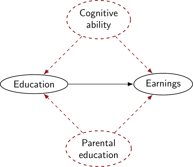
The people who stay in school longer differ systematically:

• Cognitive ability — raises schooling and earnings.
• Parental education and money — raises both.
• Ambition, health, networks — the list does not end.

Beware: this is textbook ability bias. Both confounders push the same way, so the naïve OLS estimate should be too large.

Use last week’s sign rule out loud: both arrows into education are positive, both arrows into earnings are positive, so the omitted variable bias is positive and OLS should overstate the return. Get them to commit to that prediction — it makes the actual result later genuinely surprising, and the surprise is where the real teaching happens.

Why not just control for ability?

Last week’s answer would be: measure the confounders and control for them.

Discuss: what goes wrong if we try that here?

“Ability” is not in the data — and no test score fully captures it. Ambition, family connections, health are worse still. Multiple OLS can only close the backdoors you measured, and here the important ones are invisible.

\(\rightarrow\) We need variation in schooling that has nothing to do with who the person is.

This is the hinge between L8 and today, so let them try the obvious answer first. The point to land: controlling is not wrong here, it is insufficient — the decisive confounders were never recorded, and no amount of regression conjures them back. That is precisely the situation an instrument is built for.

Angrist and Krueger (1991) had an idea

In the US at the time:

• The school year starts in September; children enter in the calendar year they turn 6.
• School is compulsory until the 16th birthday.

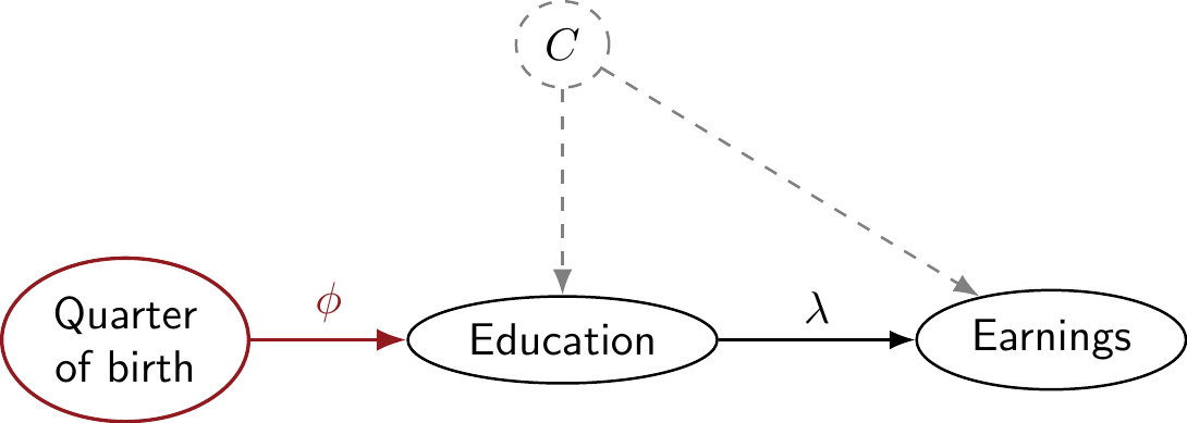
\(\rightarrow\) Children born late in the year start school younger, so they have completed more schooling by the time they may legally drop out.

Carl — born 1 January	starts aged 6½, drops out at 16 with 9 years
Luis — born 31 December	starts aged 5½, drops out at 16 with 10 years

Discuss: is quarter of birth a valid instrument? Check all three requirements from Lecture 7.

Tell the Carl and Luis story properly — it is what makes the design click, and students remember the two boys long after they forget the algebra. Then run the three requirements as a genuine check, not a recital: first stage (plausible, and we will measure it), as-if random (nobody chooses their birth quarter — or do they? hold that thought for Part 3), exclusion restriction (the one that will occupy the rest of the lecture).

Preparation

• Packages
• The data
• Why logged wages?

pacman::p_load(
  tidyverse,        # Data manipulation and visualization
  estimatr,         # OLS with robust standard errors
  modelr,           # Predictions and residuals from a model
  ivreg,            # IV / two-stage least squares
  modelsummary,     # Nicely formatted regression tables
  masteringmetrics  # The data behind Mastering 'Metrics
)

# 329,509 US men born 1930-1939, from the 1980 Census
data("ak91", package = "masteringmetrics")

ak91 %>%
  select(lnw, s, yob, qob) %>%
  head(4)
# # A tibble: 4 × 4
#     lnw     s   yob   qob
#   <dbl> <int> <int> <dbl>
# 1  5.79    12  1930     1
# 2  5.95    11  1930     1
# 3  5.32    12  1930     1
# 4  5.60    12  1930     1

lnw = log weekly wage · s = years of schooling · yob = year of birth · qob = quarter of birth.

The outcome is the log of the wage, so a coefficient reads as an approximate percentage change: a coefficient of \(0.07\) means an extra year of schooling goes with about 7% higher earnings.

This is the standard convention in the returns-to-education literature — you will meet it in every paper on the topic.

Keep this brief. Two things they must carry forward: the outcome is logged, so coefficients read as percentages, and the sample is large — 330,000 men — which will matter when we discuss how a tiny effect can still be statistically significant. Do not dwell; the payoff is next.

The naïve answer

# Just regress log wage on years of schooling
ols <- lm_robust(lnw ~ s, data = ak91)

modelsummary(
  list("log wage" = ols),
  coef_rename = c("s" = "Years of schooling"),
  stars = TRUE, gof_map = c("nobs", "r.squared"),
  output = "kableExtra"
)

Discuss: we predicted ability bias makes this too large. Hold that thought.

	log wage
(Intercept)	4.995***
	(0.005)
Years of schooling	0.071***
	(0.000)
Num.Obs.	329509
R2	0.117
+ p < 0.1, * p < 0.05, ** p < 0.01, *** p < 0.001

An extra year of schooling goes with about 7.1% higher weekly wages. Descriptively solid — causally, contaminated by every confounder we just listed.

Read the number in words and in percent. Remind them of their own prediction — ability bias means this 7.1% should be an overstatement, so the honest causal effect ought to come out lower. Write “7.1%” on the board; the whole rest of the lecture is a test of that prediction, and it will not go the way they expect.

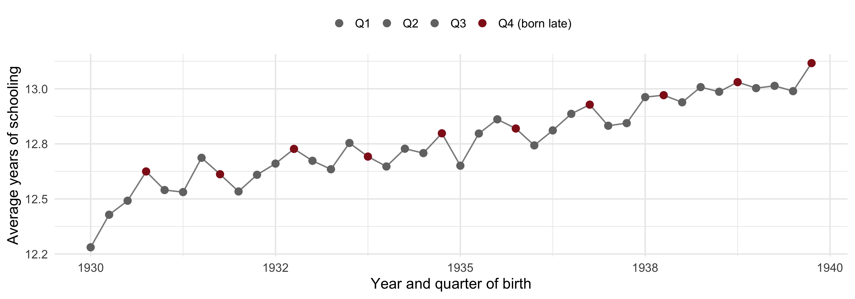
The first stage, drawn

Discuss: the line saw-tooths. What is systematically different about the red points — and is that a pattern a confounder could produce?

This is the single most persuasive slide in the lecture, so let them look before you talk. Within almost every birth year the Q4 men have more schooling than the Q1 men born a few months later — a regular sawtooth, repeated across a decade. Then the rhetorical move: what confounder could possibly generate a pattern that resets every January? That regularity is the argument for as-if randomness. Also flag how small the steps are on the y-axis; that comes back in Part 3.

Recap: first stage, reduced form, Wald

• The three quantities
• First stage in R
• Reduced form in R

First stage — does the instrument move the treatment? \[\phi = \text{Avg}[D \mid Z = 1] - \text{Avg}[D \mid Z = 0]\]

Reduced form — does the instrument move the outcome? \[\rho = \text{Avg}[Y \mid Z = 1] - \text{Avg}[Y \mid Z = 0]\]

Wald IV estimator — the effect of the treatment itself: \[\lambda = \frac{\rho}{\phi}\]

Exactly the logic from Lecture 7’s Moving to Opportunity study — only the application is new.

# Does quarter of birth move schooling?
first_stage <- lm_robust(s ~ qob, data = ak91)

modelsummary(list("Years of schooling" = first_stage),
             coef_rename = c("qob" = "Quarter of birth"),
             stars = TRUE, gof_map = c("nobs"), output = "kableExtra")

	Years of schooling
(Intercept)	12.641***
	(0.014)
Quarter of birth	0.052***
	(0.005)
Num.Obs.	329509
+ p < 0.1, * p < 0.05, ** p < 0.01, *** p < 0.001

# Does quarter of birth move wages?
reduced_form <- lm_robust(lnw ~ qob, data = ak91)

modelsummary(list("log wage" = reduced_form),
             coef_rename = c("qob" = "Quarter of birth"),
             stars = TRUE, gof_map = c("nobs"), output = "kableExtra")

	log wage
(Intercept)	5.887***
	(0.003)
Quarter of birth	0.005***
	(0.001)
Num.Obs.	329509
+ p < 0.1, * p < 0.05, ** p < 0.01, *** p < 0.001

Deliberate repetition from Lecture 7 — say so, so they know it is a recap and not something new. Have them read both coefficients aloud with units: a quarter later in the year buys about 0.05 extra years of schooling and about half a percent more in wages. Both are tiny; the ratio is not. Stress the order of operations, because students reliably invert the fraction.

The Wald answer

\[\lambda = \frac{\rho}{\phi} = \frac{0.00512}{0.0516} = \mathbf{0.0992}\]

So the causal return to a year of schooling is about 9.9%.

Discuss: we predicted ability bias would make OLS too large. OLS gave 7.1%, IV gives 9.9%. That is the wrong way round. What could explain it?

Three honest possibilities:

1. LATE, not ATE (L7) — IV identifies the effect among compliers: men who left school the moment they legally could. Returns may genuinely be higher for them.

2. Measurement error in self-reported schooling biases OLS toward zero; IV is immune to it.

3. The instrument is weak — which we come back to in Part 3.

The surprise, and it is a gift — do not smooth it over. Their sign prediction was reasonable and the data contradicted it, which is exactly what a real research finding feels like. Give them a minute on the blue box before revealing. All three explanations are live in the literature; the complier story is the one they can already reason about from Lecture 7, so lead with it.

Two-stage least squares

Part 2 of 3

The Wald ratio is a dead end the moment you want to add a control. 2SLS is the same idea, rebuilt to scale — and it is Frisch–Waugh in mirror image.

What Wald cannot do

The Wald ratio is two group means divided by two group means. That is all it can ever be.

It breaks down as soon as you want to:

• control for something (year of birth, state of birth);
• use more than one instrument;
• instrument a continuous treatment properly.

2SLS gets all three — and, with a single instrument and no controls, returns precisely the Wald number. Nothing is lost by switching.

This is why every IV paper you will ever read reports 2SLS, and why ivreg() is the function to learn.

Motivate the new tool by the limitation, not by novelty. Ask why controls might matter here even with a good instrument — year and state of birth are the obvious answers, since schooling laws and economic conditions differ across both. Then promise the reassurance: switching to 2SLS costs them nothing, because it reproduces Wald exactly in the simple case.

Stage one: keep the predicted part

Regress the treatment on the instrument — then keep the predictions, not the residuals:

first_stage <- lm_robust(s ~ qob, data = ak91)

ak91 <- ak91 %>%
  add_predictions(first_stage, var = "pred_s") %>%
  add_residuals(first_stage,  var = "e_s")

Discuss: last week we kept the residuals. Today we keep the predictions. Which of the two is unconfounded here — and why is it the opposite of last week?

pred_s — the part of schooling driven by quarter of birth, and therefore by nothing else. e_s is everything else about a person’s schooling, ability and family included.

Last week the confounder was the nuisance, so we threw its part away. Today the instrument is the only trustworthy part, so we throw everything else away.

The conceptual heart of the lecture, and the payoff of last week’s Frisch–Waugh. Make them answer before revealing. The inversion is what confuses people: with a control we discard the predicted part and keep the residuals; with an instrument we discard the residuals and keep the predicted part. Same machinery, opposite half retained — because a confounder is contamination whereas an instrument is the only clean variation in the room.

Stage two: use it as the predictor

Now regress the outcome on those predictions:

\[\text{Stage 1:}\quad D_i = \alpha_1 + \phi Z_i + e_i\] \[\text{Stage 2:}\quad Y_i = \alpha_2 + \lambda_{\text{2SLS}} \widehat{D}_i + e_i\]

second_stage <- lm_robust(lnw ~ pred_s, data = ak91)

Beware: never do this by hand in real work — the standard errors from a manual second stage are wrong, because they ignore that \(\widehat{D}\) was itself estimated. We do it here only to see the machinery.

# The same thing, done properly, in one line
iv <- ivreg(lnw ~ s | qob, data = ak91) #<<

modelsummary(
  list("OLS" = ols, "2nd stage by hand" = second_stage, "ivreg (2SLS)" = iv),
  coef_map = c("s" = "Years of schooling",
               "pred_s" = "Years of schooling (predicted)"),
  stars = TRUE, gof_map = c("nobs"), output = "kableExtra"
)

	OLS	 2nd stage by hand	 ivreg (2SLS)
Years of schooling	0.071***		0.099***
	(0.000)		(0.020)
Years of schooling (predicted)		0.099***
		(0.021)
Num.Obs.	329509	329509	329509
+ p < 0.1, * p < 0.05, ** p < 0.01, *** p < 0.001

Walk the two equations, then show that the hand-rolled second stage and ivreg() give the same coefficient. Do not skip the warning in the margin — students love doing 2SLS manually and then report standard errors that are too small, because the second stage treats the predicted values as if they were data rather than estimates. ivreg() fixes that for them.

2SLS is Wald

\[\underbrace{0.0992}_{\text{Wald: } \rho/\phi} \;=\; \underbrace{0.0992}_{\texttt{ivreg()}}\]

To four decimal places. 2SLS does not replace the Wald estimator — it contains it, and generalises it to controls and multiple instruments.

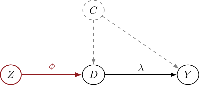
One instrument, no controls \(\rightarrow\) the two routes coincide exactly.

Put the two numbers side by side and let the identity land — this is the slide that answers “why did we bother learning Wald then?”. They bothered because Wald is where the intuition lives: a ratio of two things you can see. 2SLS is the same quantity computed in a way that scales. Nothing they learned in Lecture 7 has been discarded.

Control variables vs. instrument variables

A control \(C\) is a confounder — contamination.

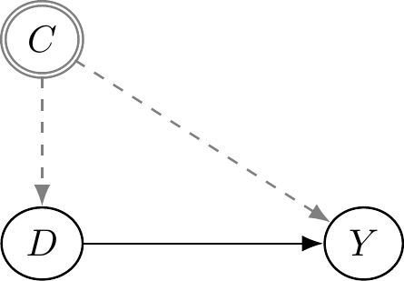
Controlling keeps the residuals of \(D\) — the part that does not correlate with \(C\).

An instrument \(Z\) is a source of random variation — the good stuff.

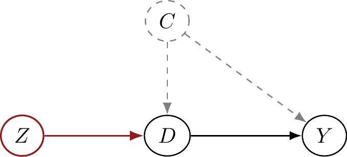
Instrumenting keeps the predicted values of \(D\) — the part that does correlate with \(Z\).

The summary slide for the whole IV/controls block — worth a full minute. Two variables, both causes of the treatment, and the correct response to each is the exact opposite. Say it as a couplet: throw the confounder’s part away, keep only the instrument’s part. If they can state that contrast cleanly they have understood both Lecture 8 and today.

Break

Your turn: exercise 1

You replicate Acemoglu & Angrist: US child-labour laws as an instrument for schooling — first stage, reduced form, Wald, then 2SLS with controls.

Open exercise 1 in a new tab ↗

The exclusion restriction

Part 3 of 3

The requirement you cannot test — and the one that has been used to demolish this very study.

Is being born in December really random?

The exclusion restriction says quarter of birth may affect earnings only through schooling.

Buckles and Hungerman (2013) checked who actually gives birth when — and found that season of birth is not random at all.

Beware: mothers giving birth in winter are, on average, younger, less educated and less likely to be married. Birth timing is partly a choice, and the kind of family that makes it differs.

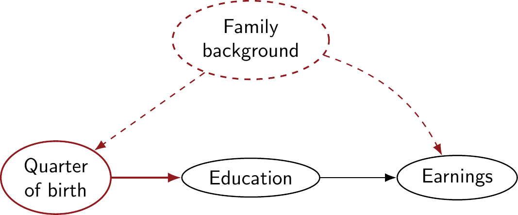
If family background causes both birth timing and earnings, the red path bypasses education entirely.

The best critique in the course, and worth teaching as a model of how scholarship actually works: a famous design, taken apart a decade later by people who simply looked at who gives birth in which month. Trace the red path with your finger — it runs from family background to birth timing to earnings without passing through education, which is precisely what the exclusion restriction forbids. Note that this is an argument, not a test; nobody can prove the path is there.

When the exclusion restriction fails

An instrument that violates the exclusion restriction is not a weak instrument — it is a confounder.

And IV makes it worse, because the Wald ratio divides by \(\phi\):

\[\text{bias} \;\propto\; \frac{1}{\phi}\]

Here \(\phi = 0.0516\) — quarter of birth shifts schooling by about 19 days. So \(1/\phi \approx 19\): any direct effect of birth timing on earnings is magnified roughly 19-fold in the IV estimate.

Discuss: with such a tiny first stage, would you rather have this instrument — or no instrument at all?

This is the weak instrument problem. A small \(\phi\) means a large \(1/\phi\), and a large \(1/\phi\) means even a trivial violation of the exclusion restriction can swamp your estimate. Weak instruments are not merely imprecise — they are fragile.

The quantitative punchline, and it is genuinely sobering. Quarter of birth moves schooling by about nineteen days, so dividing by that number multiplies everything — including any bias — roughly nineteen-fold. Make them feel the arithmetic: a violation too small to detect in the reduced form becomes a large error in the IV estimate. This is why the returns-to-education literature has argued about this instrument for thirty years, and it is the honest note to end the technical material on.

Your turn: exercise 2

You put a number on the fragility: measure the first stage, compute the amplification, and see what a hypothetical small exclusion violation would do to the estimate.

Open exercise 2 in a new tab ↗

Today’s general lessons

1. 2SLS runs IV in two steps: regress the treatment on the instrument, keep the predicted values, then use those to predict the outcome. ivreg(y ~ d | z) does both properly.

2. With one instrument and no controls, 2SLS equals the Wald ratio exactly. 2SLS earns its place by handling controls and several instruments.

3. Instrument vs. control — the mirror image: a control is contamination, so you keep the residuals; an instrument is the trustworthy variation, so you keep the predictions.

4. The exclusion restriction cannot be tested, only argued. If it fails, the instrument becomes a confounder.

5. A weak instrument (small \(\phi\)) is dangerous, not just imprecise: dividing by \(\phi\) magnifies any violation by \(1/\phi\).

Recap briskly. If one sentence survives, make it point five paired with point four: an instrument’s credibility rests on an untestable assumption, and the weaker the first stage the more damage a violation does. That is why good IV papers spend most of their pages defending the instrument rather than reporting coefficients.

Check yourself: today’s goals

• Compute a Wald estimate from a first stage and a reduced form — and say which goes on top.
• Explain what ivreg(y ~ d | z) does in two stages, and why we keep the predicted treatment rather than the residuals.
• State the exclusion restriction for quarter of birth, give one reason it might fail, and say why a small first stage makes that failure worse.

Shaky on any of these? That is what this week’s Absalon quiz and the Friday exercise class are for.

Today’s important functions

• ivreg::ivreg(y ~ d | z): two-stage least squares — treatment before the |, instrument after it.
• ivreg(y ~ d + c | z + c): 2SLS with controls — note the controls appear on both sides.
• modelr::add_predictions(model, var = ...): keep the fitted values (the first stage of 2SLS by hand).
• modelr::add_residuals(model, var = ...): keep the residuals (what controlling keeps instead).
• lm_robust(d ~ z) / lm_robust(y ~ z): the first stage and the reduced form.

References

Angrist, J. D. and A. B. Krueger (1991). “Does Compulsory School Attendance Affect Schooling and Earnings?*“. In: The Quarterly Journal of Economics, pp. 979-1014.

Buckles, K. S. and D. M. Hungerman (2013). “Season of Birth and Later Outcomes: Old Questions, New Answers”. In: The Review of Economics and Statistics, pp. 711-724.